1. ENTX 1000; STX X.
2. The STJ instruction in line 03 resets this address. (It is conventional to denote the address of such instructions by ‘*’, both because it is simple to write, and because it provides a recognizable test of an error condition in a program, in case a subroutine has not been entered properly because of some oversight. Some people prefer ‘*-*’.)
3. Read in 100 words from tape unit zero; exchange their maximum with the last of them; exchange the maximum of the remaining 99 with the last of those; etc. Eventually the 100 words will become completely sorted into nondecreasing order. The result is then written onto tape unit one. (Compare with Algorithm 5.2.3S.)
4. Nonzero locations:
5. Each OUT waits for the previous printer operation to finish (from the other buffer).
6. (a) If n is not prime, by definition n has a divisor d with $1\lt d\lt n$. If $d\gt\sqrt{n}$, then $n/d$ is a divisor with $1\lt{n/d}\lt\sqrt{n}$. (b) If N is not prime, N has a prime divisor d with $1\lt{d}\le\sqrt{\tt N}$. The algorithm has verified that N has no prime divisors $≤ p=\tt PRIME[K]$; also ${\tt N}=p{\tt Q}+{\tt R}\lt p{\tt Q}+p≤p^{2}+p\lt (p+1)^{2}$. Any prime divisor of N is therefore greater than $p+1\gt\sqrt{\tt N}$.
We must also prove that there will be a sufficiently large prime less than N when N is prime, namely that the $(k+1)$st prime $p_{k+1}$ is less than $p_{k}^{2}+p_{k}$ otherwise K would exceed J and $\tt PRIME[K]$ would be zero when we needed it to be large. The necessary proof follows from “Bertrand’s postulate”: If p is prime there is a larger prime less than 2p.
7. (a) It refers to the location of line 29. (b) The program would then fail; line 14 would refer to line 15 instead of line 25; line 24 would refer to line 15 instead of line 12.
8. It prints 100 lines. If the 12000 characters on these lines were arranged end to end, they would reach quite far and would consist of five blanks followed by five A’s followed by ten blanks followed by five A’s followed by fifteen blanks ... followed by 5k blanks followed by five A’s followed by $5(k+1)$ blanks ... until 12000 characters have been printed. The third-from-last line ends with AAAAA and 35 blanks; the final two lines are entirely blank. The total effect is one of OP art.
9. The (4:4) field of each entry in the following table holds the maximum F setting; the (1:2) field is the location of an appropriate validity-check routine.

10. The catch to this problem is that there may be several places in a row or column where the minimum or maximum occurs, and each is a potential saddle point.
Solution 1: In this solution we run through each row in turn, making a list of all columns in which the row minimum occurs and then checking each column on the list to see if the row minimum is also a column maximum. rX ≡ current min; rI1 traces through the matrix, going from 72 down to zero unless a saddle point is found; rI2 ≡ column index of rI1; rI3 ≡ size of list of minima. Notice that in all cases the terminating condition for a loop is that an index register is ≤ 0.

Solution 2: An infusion of mathematics gives a different algorithm.
Theorem. Let $R(i)=\min_{j} a_{ij}$, $C(j)=\max_{i} a_{ij}$. The element $a_{\large i_{0}j_{0}}$ is a saddle point if and only if $R(i_{0})=\max_{i} R(i)=C(j_{0})=\min_{j} C(j)$.
Proof. If $a_{\large i_{0}j_{0}}$ is a saddle point, then for any fixed i, $R(i_{0})=C(j_{0})≥a_{ij_{0}}≥R(i)$; so $R(i_{0})=\max_{i} R(i)$. Similarly $C(j_{0})=\min_{j} C(j)$. Conversely, we have $R(i)≤a_{ij}≤C(j)$ for all i and j; hence $R(i_{0})=C(j_{0})$ implies that $a_{\large i_{0}j_{0}}$ is a saddle point. 
(This proof shows that we always have $\max_{i} R(i) ≤\min_{j} C(j)$. So there is no saddle point if and only if all the R’s are less than all the C’s.)
According to the theorem, it suffices to find the smallest column maximum, then to search for an equal row minimum. During Phase 1, rI1 ≡ column index; rI2 runs through the matrix. During Phase 2, rI1 ≡ possible answer; rI2 runs through the matrix; rI3 ≡ row index times 8; rI4 ≡ column index.
We leave it to the reader to invent a still better solution in which Phase 1 records all possible rows that are candidates for the row search in Phase 2. It is not necessary to search all rows, just those $i_{0}$ for which $C(j_{0})=\min_{j} C(j)$ implies $a_{\large i_{0}j_{0}}=C(j_{0})$. Usually there is at most one such row.
In some trial runs with elements selected at random from $\{0,1,2,3,4\}$, solution 1 required approximately 730u to run, while solution 2 took about 530u. Given a matrix of all zeros, solution 1 found a saddle point in 137u, solution 2 in 524u.
If an $m\times n$ matrix has distinct elements, and m ≥ n, we can solve the problem by looking at only $O(m+n)$ of them and doing $O(m\log n)$ auxiliary operations. See Bienstock, Chung, Fredman, Schäffer, Shor, and Suri, AMM 98 (1991), 418–419.
11. Assume an $m\times n$ matrix. (a) By the theorem in the answer to exercise 10, all saddle points of a matrix have the same value, so (under our assumption of distinct elements) there is at most one saddle point. By symmetry the desired probability is mn times the probability that $a_{11}$ is a saddle point. This latter is $1/(mn)!$ times the number of permutations with $a_{12}\gt a_{11},\ldots,a_{1n}\gt a_{11},a_{11}\gt a_{21},\ldots,a_{11}\gt a_{m1}$; this is $1/(m+n-1)!$ times the number of permutations of $m+n-1$ elements in which the first is greater than the next $(m-1)$ and less than the remaining $(n-1)$, namely $(m-1)! (n-1)!$. The answer is therefore

In our case this is $17/\mybinomf{17}{8}$, only one chance in 1430. (b) Under the second assumption, an entirely different method must be used. The probability equals the probability that there is a saddle point with value zero plus the probability that there is a saddle point with value one. The former is the probability that there is at least one column of zeros; the latter is the probability that there is at least one row of ones. The answer is $(1-(1-2^{-m})^{n})+(1-(1-2^{-n})^{m})$; in our case it comes to $924744796234036231/18446744073709551616$, about 1 in $19.9$. An approximate answer is $n2^{-m}+m2^{-n}$.
12. M. Hofri and P. Jacquet [Algorithmica 22 (1998), 516–528] have analyzed the case when the $m\times n$ matrix entries are distinct and in random order. The running times of the two MIX programs are then respectively $(6mn+5mH_{n}+8m+6+5(m+1)/(n-1))u+O{\big(}(m+n)^{2}/\mybinomf{m+n}{m}{\big)}$ and $(5mn+2nH_{m}+7m+7n+9H_{n})u+$ $O(1/n)+O((\log n)^{2}/m)$, as $m→∞$ and $n→∞$, assuming that $(\log n)/m→0$.
13.


For this problem, buffering of output is not desirable since it could save at most 7u of time per line output.
14. To make the problem more challenging, the following solution due in part to J. Petolino uses a lot of trickery in order to reduce execution time. Can the reader squeeze out any more microseconds?


A rigorous justification for the change from division to multiplication in several places can be based on the fact that the number in rA is not too large. The program works with all byte sizes.
[To calculate Easter in years ≤ 1582, see CACM 5 (1962), 209–210. The first systematic algorithm for calculating the date of Easter was the canon paschalis due to Victorius of Aquitania (A.D. 457). There are many indications that the sole nontrivial application of arithmetic in Europe during the Middle Ages was the calculation of Easter date, hence such algorithms are historically significant. See Puzzles and Paradoxes by T. H. O’Beirne (London: Oxford University Press, 1965), Chapter 10, for further commentary; and see the book Calendrical Calculations by E. M. Reingold and N. Dershowitz (Cambridge Univ. Press, 2001) for date-oriented algorithms of all kinds.]
15. The first such year is A.D. 10317, although the error almost leads to failure in A.D. 10108 + 19k for 0 ≤ k ≤ 10.
Incidentally, T. H. O’Beirne pointed out that the date of Easter repeats with a period of exactly 5,700,000 years. Calculations by Robert Hill show that the most common date is April 19 (220400 times per period), while the earliest and least common is March 22 (27550 times); the latest, and next-to-least common, is April 25 (42000 times). Hill found a nice explanation for the curious fact that the number of times any particular day occurs in the period is always a multiple of 25.
16. Work with scaled numbers, $R_{n}=10^{n}r_{n}$. Then $R_{n} (1/m)=R$ if and only if $10^{n}/(R+\frac12)\lt{m}\le10^{n}/(R-\frac12)$; thus we find $m_{h}=\lfloor{2·10^{n}/(2R-1)}\rfloor$.


0006.16 0008.449 0010.7509 0013.05363
in 65595u plus output time. (It would be faster to calculate $R_{n} (1/m)$ directly when $m\lt{10^{n/2}\sqrt{2}}$, and then to apply the suggested procedure.)
17. Let $N=\lfloor 2·10^{n}/(2m+1)\rfloor$. Then $S_{n}=H_{N}+O(N/10^{n})+∑_{k=1}^{m}(\lfloor2·10^{n}/(2k-1)\rfloor-\lfloor2·10^{n}/(2k+1)\rfloor)k/10^{n}=$ $H_{N}+O(m^{-1})+O(m/10^{n})-1+2H_{2m}-H_{m}=$ $n\ln{10}+2\gamma-1+2\ln{2}+O(10^{-n/2})$ if we sum by parts and set $m ≈ 10^{n/2}$.
Incidentally, the next several values are $S_{6}=15.356262$, $S_{7}=17.6588276$, $S_{8}=19.96140690$, $S_{9}=22.263991779$, and $S_{10}=24.5665766353$; our approximation to $S_{10}$ is $≈24.566576621$, which is closer than predicted.
18.

19. (a) Induction. (b) Let k ≥ 0 and $X=ax_{k+1}-x_{k}$, $Y=ay_{k+1}-y_{k}$, where $a=\lfloor(y_{k}+n)/y_{k+1}\rfloor$. By part (a) and the fact that 0 < Y ≤ n, we have $X⊥Y$ and $X/Y\gt x_{k+1}/y_{k+1}$. So if $X/Y≠x_{k+2}/y_{k+2}$ we have, by definition, $X/Y\gt x_{k+2}/y_{k+2}$. But this implies that

Historical notes: C. Haros gave a (more complicated) rule for constructing such sequences, in J. de l’École Polytechnique 4, 11 (1802), 364–368; his method was correct, but his proof was inadequate. Several years later, the geologist John Farey independently conjectured that $x_{k}/y_{k}$ is always equal to $(x_{k-1}+x_{k+1})/(y_{k-1}+y_{k+1})$ [Philos. Magazine and Journal 47 (1816), 385–386]; a proof was supplied shortly afterwards by A. Cauchy [Bull. Société Philomathique de Paris (3) 3 (1816), 133–135], who attached Farey’s name to the series. For more of its interesting properties, see G. H. Hardy and E. M. Wright, An Introduction to the Theory of Numbers, Chapter 3.
20.


22.


The last man is in position 15. The total time before output is $(4(N-1)(M+7.5)+16)u$. Several improvements are possible, such as D. Ingalls’s suggestion to have three-word packets of code ‘DEC2 1; J2P NEXT; JMP OUT’, where OUT modifies the NEXT field so as to delete a packet. An asymptotically faster method appears in exercise 5.1.1–5.
1. $(1\;2\;4)(3\;6\;5)$.
2. $a↔c$, $c↔f$; $b↔d$. The generalization to arbitrary permutations is clear.
3. $\left(\begin{myarray1}a&b&c&d&e&f\\d&b&f&c&a&e\end{myarray1}\right)$.
4. $(a\;d\;c\;f\;e)$.
5. 12. (See exercise 20.)
6. The total time decreases by 8u for every blank word following a “(”, because lines 30–32 cost 4u while lines 26–28, 33–34, 36–38 cost 12u. It decreases by 2u for every blank word following a name, because lines 68–71 cost 5u while 42–46 or 75–79 cost 7u. Initial blanks and blanks between cycles do not affect the execution time. The position of blanks has no effect whatever on Program B.
7. X = 2, Y = 29, M = 5, N = 7, U = 3, V = 1. Total, by Eq. (18), 2161u.
8. Yes; we would then keep the inverse of the permutation, so that $x_{i}$ goes to $x_{j}$ if and only if $T[j]=i$. (The final cycle form would then be constructed from right to left, using the T table.)
9. No. For example, given (6) as input, Program A will produce ‘$({\tt ADG})({\tt CEB})$’ as output, while Program B produces ‘$({\tt CEB})({\tt DGA})$’. The answers are equivalent but not identical, due to the nonuniqueness of cycle notation. The first element chosen for a cycle is the leftmost available name, in the case of Program A, and the last available distinct name to be encountered from right to left, in Program B.
10. (1) Kirchhoff’s law yields $A=1+C-D$; $B=A+J+P-1$; $C=B-(P-L)$; $E=D-L$; $G=E$; $Q=Z$; $W=S$. (2) Interpretations: B = number of words of input = 16X − 1; C = number of nonblank words = Y; D = C − M; E = D − M; F = number of comparisons in names table search; H = N; K = M; Q = N; R = U; S = R − V; T = N − V since each of the other names gets tagged. (3) Summing up, we have $(4F+16Y+80X+21N-19M+9U-16V)u$, which is somewhat better than Program A because F is certainly less than 16NX. The time in the stated case is 983u, since F = 74.
11. “Reflect” it. For example, the inverse of $(a\;c\;f)(b\;d)$ is $(d\;b)(f\;c\;a)$.
12. (a) The value in cell $L+mn-1$ is fixed by the transposition, so we may omit it from consideration. Otherwise if $x=n(i-1)+(j-1)\lt mn-1$, the value in L + x should go to cell $L+mx\bmod N=L+(mn(i-1)+m(j-1))\bmod N=L+m(j-1)+(i-1)$, since $mn≡\md[1]{N}$ and $0≤m(j-1)+(i-1)\lt N$. (b) If one bit in each memory cell is available (for example, the sign), we can “tag” elements as we move them, using an algorithm like Algorithm I. [See M. F. Berman, JACM 5 (1958), 383–384.] If there is no room for a tag bit, tag bits can be kept in an auxiliary table, or else a list of representatives of all non-singleton cycles can be used: For each divisor d of N, we can transpose those elements that are multiples of d separately, since m is prime to N. The length of the cycle containing x, when $\gcd(x,N)=d$, is the smallest integer r > 0 such that $m^{r}≡\md[1]{N/d}$. For each d, we want to find $φ(N/d)/r$ representatives, one from each of these cycles. Some number-theoretic methods are available for this purpose, but they are not simple enough to be really satisfactory. An efficient but rather complicated algorithm can be obtained by combining number theory with a small table of tag bits. [See N. Brenner, CACM 16 (1973), 692–694.] Finally, there is a method analogous to Algorithm J; it is slower, but needs no auxiliary memory, and it performs any desired permutation in situ. [See P. F. Windley, Comp. J. 2 (1959), 47–48; D. E. Knuth, Proc. IFIP Congress (1971), 1, 19–27; E. G. Cate and D. W. Twigg, ACM Trans. Math. Software 3 (1977), 104–110; F. E. Fich, J. I. Munro, and P. V. Poblete, SICOMP 24 (1995), 266–278.]
13. Show by induction that, at the beginning of step J2, $X[i]=+j$ if and only if j > m and j goes to i under π; $X[i]=-j$ if and only if i goes to j under $π^{k+1}$, where k is the smallest nonnegative integer such that $π^{k}$ takes i into a number ≤ m.
14. Writing the inverse of the given permutation in canonical cycle form and dropping parentheses, the quantity A − N is the sum of the number of consecutive elements greater than a given element and immediately to its right. For example, if the original permutation is $(1\;6\;5)(3\;7\;8\;4)$, the canonical form of the inverse is $(3\;4\;8\;7)(2)(1\;5\;6)$; set up the array

and the quantity A is the number of “dots,” 16. The number of dots below the kth element is the number of right-to-left minima in the first k elements (there are 3 dots below 7 in the example above, since there are 3 right-to-left minima in 3487). Hence the average is $H_{1}+H_{2}+\cdots+H_{n}=(n+1)H_{n}-n$.
15. If the first character of the linear representation is 1, the last character of the canonical representation is 1. If the first character of the linear representation is m > 1, then “$\ldots 1m\ldots$” appears in the canonical representation. So the only solution is the permutation of a single object. (Well, there’s also the permutation of no objects.)
16. 1324, 4231, 3214, 4213, 2143, 3412, 2413, 1243, 3421, 1324, ....
17. (a) The probability $p_{m}$ that the cycle is an m-cycle is $n!/m$ divided by $n! H_{n}$, so $p_{m}=1/(mH_{n})$. The average length is  . (b) Since the total number of m-cycles is $n!/m$, the total number of appearances of elements in m-cycles is $n!$. Each element appears as often as any other, by symmetry, so k appears $n!/n$ times in m-cycles. In this case, therefore, $p_{m}=1/n$ for all k and m; the average is
  .
.
18. See exercise 22(e).
19. $|P_{n0}-n!/e|=n!/(n+1)!-n!/(n+2)!+\cdots$, an alternating series of decreasing magnitudes, which is less than  .
.
20. There are $α_{1}+α_{2}+\cdots$ cycles in all, which can be permuted among one another, and each m-cycle can be independently written in m ways. So the answer is
$(α_{1}+α_{2}+\cdots)! 1^{α_{1}} 2^{α_{2}} 3^{α_{3}}\ldots.$
21. $1/(α_{1}!1^{α_{1}} α_{2}! 2^{α_{2}}\ldots)$ if $n=α_{1}+2α_{2}+\cdots$; zero otherwise.
Proof. Write out $α_{1}$ 1-cycles, $α_{2}$ 2-cycles, etc., in a row, with empty positions; for example if $α_{1}=1,α_{2}=2,α_{3}=α_{4}=\cdots=0$, we would have “$\tt(-)(--)(--)$”. Fill the empty positions in all n! possible ways; we obtain each permutation of the desired form exactly $α_{1}!1^{α_{1}} α_{2}!2^{α_{2}}\ldots$ times.
22. (a) If $k_{1}+2k_{2}+\cdots=n$, the probability in (ii) is $∏_{j\gt 0}f(w,j,k_{j})$, which is assumed to equal $(1-w)w^{n}/(k_{1}! 1^{k_{1}}k_{2}! 2^{k_{2}}\ldots)$; hence

Therefore by induction $f(w,m,k)=(w^{m}/m)^{k}f(w,m,0)/k!$, and condition (i) implies that $f (w,m,k)=(w^{m}/m)^{k}e^{-w^{m}/m}/k!$. [In other words, $α_{m}$ is chosen with a Poisson distribution; see exercise 1.2.10–15.]
(b) 
Hence the probability that $α_{1}+2α_{2}+\cdots≤n$ is $(1-w)(1+w+\cdots+w^{n})=1-w^{n+1}$.
(c) The average of φ is

(d) Let $φ(α_{1},α_{2},\ldots)=α_{2}+α_{4}+α_{6}+\cdots$. The average value of the linear combination φ is the sum of the average values of $α_{2},α_{4},α_{6},\ldots$; and the average value of $α_{m}$ is

Therefore the average value of φ is

The desired answer is $\frac12{H_{\lfloor{n/2}\rfloor}}$.
(e) Set $φ(α_{1},α_{2},\ldots)=z^{α_{m}}$, and observe that the average value of φ is

Hence

the statistics are $(\min 0,{\rm ave}\;{1/m},\max\lfloor n/m\rfloor,{\rm dev}\sqrt{1/m})$, when n ≥ 2m.
23. The constant λ is  , where
  . See Trans. Amer. Math. Soc. 121 (1966), 340–357, where many other results are proved, in particular that the average length of the shortest cycle is approximately $e^{-γ}\ln n$. Further terms of the asymptotic representation of $l_{n}$ have been found by Xavier Gourdon [Ph.D. thesis, École Polytechnique (Paris, 1996)]; the series begins

where $ω=e^{2πi/3}$. William C. Mitchell has calculated a high-precision value of $λ=.62432\;99885\;43550\;87099\;29363\;83100\;83724\;41796+$ [Math. Comp. 22 (1968), 411–415]; no relation between λ and classical mathematical constants is known. The same constant had, however, been computed in another context by Karl Dickman in Arkiv för Mat., Astron. och Fys. 22A, 10 (1930), 1–14; the coincidence wasn’t noticed until many years later [Theor. Comp. Sci. 3 (1976), 373].
24. See D. E. Knuth, Proc. IFIP Congress (1971), 1, 19–27.
25. One proof, by induction on N, is based on the fact that when the Nth element is a member of s of the sets it contributes exactly

to the sum. Another proof, by induction on M, is based on the fact that the number of elements that are in $S_{M}$ but not in $S_{1} ∪\cdots ∪ S_{M-1}$ is

26. Let $N_{0}=N$ and let $N_{k}=∑_{1≤j_{1}\lt\cdots \lt j_{k}≤M} |S_{j_{1}} ∩\cdots ∩ S_{j_{k}}|$. Then

is the desired formula. It can be proved from the principle of inclusion and exclusion itself, or by using the method of exercise 25 together with the fact that

27. Let $S_{j}$ be the multiples of $m_{j}$ in the stated range and let $N=am_{1}\ldots m_{t}$. Then $|S_{j} ∩ S_{k}|=N/m_{j}m_{k}$, etc., so the answer is

This also solves exercise 1.2.4–30, if we let $m_{1},\ldots,m_{t}$ be the primes dividing N.
28. See I. N. Herstein and I. Kaplansky, Matters Mathematical (1974), §3.5.
29. When passing over a man, assign him a new number (starting with n + 1). Then the kth man executed is number 2k, and man number j for j > n was previously number $(2j)\bmod (2n+1)$. Incidentally, the original number of the kth man executed is $2n+1-(2n+1-2k)2^{\lfloor\lg(2n/(2n+1-2k))\rfloor}$. [Armin Shams, Proc. Nat. Computer Conf. 2002, English papers section, 2 (Mashhad, Iran: Ferdowsi University, 2002), 29–33.]
31. See CMath, Section 3.3. Let $x_{0}=jm$ and $x_{i+1}=(m(x_{i}-n)-d_{i})/(m-1)$, where $1≤d_{i}\lt m$. Then $x_{k}=j$ if and only if $a_{k}j=b_{k}n+t_{k}$, where $a_{k}=m^{k+1}-(m-1)^{k}$, $b_{k}=m(m^{k}-(m-1)^{k})$, and $t_{k}=∑_{i=0}^{k-1}m^{k-1-i}(m-1)^{i}d_{i}$. Since $a_{k}⊥b_{k}$ and the $(m-1)^{k}$ possibilities for $t_{k}$ are distinct, the average number of k-step fixed elements is $(m-1)^{k}/a_{k}$.
32. (a) In fact, $k-1≤π_{k}≤k+2$ when k is even; $k-2≤π_{k}≤k+1$ when k is odd. (b) Choose the exponents from left to right, setting $e_{k}=1$ if and only if k and k + 1 are in different cycles of the permutation so far. [Steven Alpern, J. Combinatorial Theory B25 (1978), 62–73.]
33. For l = 0, let $(α_{01},α_{02}; β_{01},β_{02})=(π,ρ;\epsilon,\epsilon)$ and $(α_{11},α_{12}; β_{11},β_{12})=(\epsilon,\epsilon; π,ρ)$, where $π=(1\;4)(2\;3)$, $ρ=(1\;5)(2\;4)$, and $\epsilon=()$.
Suppose we have made such a construction for some l ≥ 0, where $\alpha_{jk}^{2}=\beta_{jk}^{2}=()$ for 0 ≤ j < m and 1 ≤ k ≤ n. Then the permutations
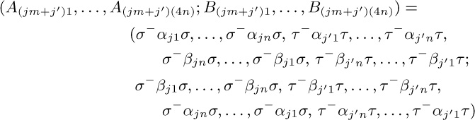
have the property that

if i = j and i′ = j′, otherwise the product is (). Choosing $σ=(2\;3)(4\;5)$ and $τ=(3\;4\;5)$ will make the product $(1\;2\;3\;4\;5)$ as desired, when $im+i′=jm+j′$.
The construction that leads from l to l + 1 is due to David A. Barrington [J. Comp. Syst. Sci. 38 (1989), 150–164], who proved a general theorem by which any Boolean function can be represented as a product of permutations of $\{1,2,3,4,5\}$. With a similar construction we can, for example, find sequences of permutations $(α_{j1},\ldots,α_{jn}; β_{j1},\ldots,β_{jn})$ such that

for $0≤i,j\lt m=2^{\large 2^{l}}$ when $n=6^{l+1}-4^{l+1}$.
34. Let $N=m+n$. If $m⊥n$ there is only one cycle, because every element can be written in the form $am mod N$ for some integer a. And in general if $d=\gcd(m,n)$, there are exactly d cycles $C_{0},C_{1},\ldots,C_{d-1}$, where $C_{j}$ contains the elements $\{j,j+d,\ldots,j+N-d\}$ in some order. To carry out the permutation, we can therefore proceed as follows for 0 ≤ j < d (in parallel, if convenient): Set $t←x_{j}$ and $k←j$; then while $(k+m)\bmod N≠j$, set $x_{k}←x_{(k+m)\bmod N}$ and $k←(k+m)\bmod N$; finally set $x_{k}←t$. In this algorithm the relation $(k+m)\bmod N≠j$ will hold if and only if $(k+m)\bmod N≥d$, so we can use whichever test is more efficient. [W. Fletcher and R. Silver, CACM 9 (1966), 326.]
35. Let $M=l+m+n$ and $N=l+2m+n$. The cycles for the desired rearrangement are obtained from the cycles of the permutation on $\{0,1,\ldots,N-1\}$ that takes k to $(k+l+m)\bmod N$, by simply striking out all elements of each cycle that are ≥ M. (Compare this behavior with the similar situation in exercise 29.) Proof: When the hinted interchange sets $x_{k}←x_{k'}$ and $x_{k'}←x_{k''}$ for some k with $k'=(k+l+m)\bmod N$ and $k''=(k'+l+m)\bmod N$ and $k'≥M$, we know that $x_{k'}=x_{k''}$; hence the rearrangement $αβγ→γβα$ replaces $x_{k}$ by $x_{k''}$.
It follows that there are exactly $d=\gcd(l+m,m+n)$ cycles, and we can use an algorithm similar to the one in the previous exercise.
A slightly simpler way to reduce this problem to the special case in exercise 34 is also noteworthy, although it makes a few more references to memory: Suppose $γ=γ'γ''$ where $|γ''|=|α|$. Then we can change $αβγ'γ''$ to $γ''βγ'α$, and interchange $γ''β$ with $γ'$. A similar approach works if $|α|\gt |γ|$. [See J. L. Mohammed and C. S. Subi, J. Algorithms 8 (1987), 113–121.]
37. The result is clear when n ≤ 2. Otherwise we can find $a,b\lt n$ such that π takes a to b. Then $(n\;a) π (b\;n)=(α\;a)(b\;β)$ for (n− 1)-cycles $(α\;a)$ and $(b\;β)$ if and only if $π=(n\;α\;a)(b\;β\;n)$. [See A. Jacques, C. Lenormand, A. Lentin, and J.-F. Perrot, Comptes Rendus Acad. Sci. 266 (Paris, 1968), A446–A448.]
1.
2.

3.
(The analogous exercise for (9) would of course be somewhat more complicated.)
4.

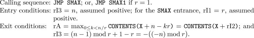
5. Any other register can be used. For example,
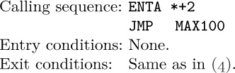
The code is like (1), but the first instruction becomes ‘$\tt MAX100\;STA\;EXIT(0\colon2)$’.
6. (Solution by Joel Goldberg and Roger M. Aarons.)

7. (1) An operating system can allocate high-speed memory more efficiently if program blocks are known to be “read-only.” (2) An instruction cache in hardware will be faster and less expensive if instructions cannot change. (3) Same as (2), with “pipeline” in place of “cache.” If an instruction is modified after entering a pipeline, the pipeline needs to be flushed; the circuitry needed to check this condition is complex and time-consuming. (4) Self-modifying code cannot be used by more than one process at once. (5) Self-modifying code can defeat a jump-trace routine (exercise 1.4.3.2–7), which is an important diagnostic tool for “profiling” (that is, for computing the number of times each instruction is executed).
1. If one coroutine calls the other only once, it is nothing but a subroutine; so we need an application in which each coroutine calls the other in at least two distinct places. Even then, it is often easy to set some sort of switch or to use some property of the data, so that upon entry to a fixed place within one coroutine it is possible to branch to one of two desired places; again, nothing more than a subroutine would be required. Coroutines become correspondingly more useful as the number of references between them grows larger.
2. The first character found by IN would be lost. [We started OUT first because lines 58–59 do the necessary initialization for IN. If we wanted to start IN first, we’d have to initialize OUT by saying ‘ENT4 -16’, and clearing the output buffer if it isn’t known to be blank. Then we could make line 62 jump first to line 39.]
3. Almost true, since ‘CMPA =10=’ within IN is then the only comparison instruction of the program, and since the code for ‘.’ is 40. (!) But the comparison indicator isn’t initialized; and if the final period is preceded by a replication digit, it won’t be noticed. [Note: The most nitpickingly efficient program would probably remove lines 40, 44, and 48, and would insert ‘CMPA PERIOD’ between lines 26 and 27, ‘CMPX PERIOD’ between lines 59 and 60. The state of the comparison indicator should then become part of the coroutine characteristics in the program documentation.]
4. Here are examples from three rather different computers of historic importance: (i) On the IBM 650, using SOAP assembly language, we would have the calling sequences ‘LDD A’ and ‘LDD B’, and linkage ‘A STD BX AX’ and ‘B STD AX BX’ (with the two linkage instructions preferably in core). (ii) On the IBM 709, using common assembly languages, the calling sequences would be ‘TSX A,4’ and ‘TSX B,4’; the linkage instructions would be as follows:

(iii) On the CDC 1604, the calling sequences would be “return jump” (SLJ 4) to A or B, and the linkage would be, for example,
A: SLJ B1; ALS 0
B: SLJ A1; SLJ A
in two consecutive 48-bit words.
5. ‘STA HOLDAIN; LDA HOLDAOUT’ between OUT and OUTX, and ‘STA HOLDAOUT; LDA HOLDAIN’ between IN and INX.
6. Within A write ‘JMP AB’ to activate B, ‘JMP AC’ to activate C. Locations BA, BC, CA, and CB would, similarly, be used within B and C. The linkage is:

[Note: With n coroutines, $2(n-1)n$ cells would be required for this style of linkage. If n is large, a “centralized” routine for linkage could of course be used; a method with 3n + 2 cells is not hard to invent. But in practice the faster method above requires just 2m cells, where m is the number of pairs $(i,j)$ such that coroutine i jumps to coroutine j. When there are many coroutines each independently jumping to others, the sequence of control is usually under external influence, as discussed in Section 2.2.5.]
1. FCHECK is used only twice, both times immediately followed by a call on MEMORY. So it would be slightly more efficient to make FCHECK a special entrance to the MEMORY subroutine, and also to make it put −R in rI2.
2.

4. Just insert ‘IN 0(16)’ and ‘JBUS *(16)’ between lines 003 and 004. (Of course on another computer this would be considerably different since it would be necessary to convert to MIX character code.)
5. Central control time is 34u, plus 15u if indexing is required; the GETV subroutine takes 52u, plus 5u if L ≠ 0; extra time to do the actual loading is 11u for LDA or LDX, 13u for LDi, 21u for ENTA or ENTX, 23u for ENTi (add 2u to the latter two times if M = 0). Summing up, we have a total time of 97u for LDA and 55u for ENTA, plus 15u for indexing, and plus 5u or 2u in certain other circumstances. It would seem that simulation in this case is causing roughly a 50:1 ratio in speeds. (Results of a test run that involved 178u of simulated time required 8422u of actual time, a 47:1 ratio.)
7. Execution of IN or OUT sets a variable associated with the appropriate input device to the time when transmission is desired. The ‘CYCLE’ control routine interrogates these variables on each cycle, to see if CLOCK has exceeded either (or both) of them; if so, the transmission is carried out and the variable is set to ∞. (When more than two I/O units must be handled in this way, there might be so many variables that it would be preferable to keep them in a sorted list using linked memory techniques; see Section 2.2.5.) We must be careful to complete the I/O when simulating HLT.
8. False; rI6 can equal BEGIN, if we “fall through” from the location BEGIN − 1. But then a MEMERROR will occur, trying to STZ into TIME! On the other hand, we always do have 0 ≤ rI6 ≤ BEGIN, because of line 254.
1. Change lines 48 and 49 to the following sequence:
The operator ‘JSJ’ here is, of course, particularly crucial.
2.

A supplementary routine that writes out the final buffer and rewinds tape 0 should be called after all tracing has been performed.
3. Tape is faster; and the editing of this information into characters while tracing would consume far too much space. Furthermore the tape contents can be selectively printed.
4. A true trace, as desired in exercise 6, would not be obtained, since restriction (a) mentioned in the text is violated. The first attempt to trace CYCLE would cause a loop back to tracing ENTER+1, because PREG is clobbered.
6. Suggestion: Keep a table of values of each memory location within the trace area that has been changed by the outer program.
7. The routine should scan the program until finding the first jump (or conditional jump) instruction; after modifying that instruction and the one following, it should restore registers and allow the program to execute all its instructions up to that point, in one burst. [This technique can fail if the program modifies its own jump instructions, or changes non-jumps into jumps. For practical purposes we can outlaw such practices, except for STJ, which we probably ought to handle separately anyway.]
1. (a) No; the input operation might not yet be complete. (b) No; the input operation might be going just a little faster than the MOVE. This proposal is much too risky.
2.
ENT1 2000
JBUS *(6)
MOVE 1000(50)
MOVE 1050(50)
OUT 2000(6)
3.

At the beginning of the program, give the instruction ‘ENT5 OUTBUF1’. At the end of the program, say

4. If the calculation time exactly equals the I/O time (which is the most favorable situation), both the computer and the peripheral device running simultaneously will take half as long as if they ran separately. Formally, let C be the calculation time for the entire program, and let T be the total I/O time required; then the best possible running time with buffering is $\max(C,T)$, while the running time without buffering is C + T; and of course $\frac12(C+T) ≤\max(C,T)≤C+T$.
However, some devices have a “shutdown penalty” that causes an extra amount of time to be lost if too long an interval occurs between references to that unit; in such a case, better than 2:1 ratios are possible. (See, for example, exercise 19.)
5. The best ratio is $(n+1)\colon\!1$.
6. 
(possibly preceded by $\tt IOC 0(U)$ to rewind the tape just in case it is necessary).
7. One way is to use coroutines:

Adding a few more instructions to take advantage of special cases will actually make this routine faster than (4).
8. At the time shown in Fig. 23, the two red buffers have been filled with line images, and the one indicated by NEXTR is being printed. At the same time, the program is computing between RELEASE and ASSIGN. When the program ASSIGNs, the green buffer indicated by NEXTG becomes yellow; NEXTG moves clockwise and the program begins to fill the yellow buffer. When the output operation is complete, NEXTR moves clockwise, the buffer that has just been printed turns green, and the remaining red buffer begins to be printed. Finally, the program RELEASEs the yellow buffer and it too is ready for subsequent printing.

and so on. Total time when N = 1 is 110000u; when N = 2 it is 89000u; when N = 3 it is 81500u; and when N ≥ 4 it is 76000u.
12. Replace the last three lines of Program B by

13.
JRED CONTROL(U)
J6NZ *-1
14. If N = 1 the algorithm breaks down (possibly referring to the buffer while I/O is in progress); otherwise the construction will have the effect that there are two yellow buffers. This can be useful if the computational program wants to refer to two buffers at once, although it ties up buffer space. In general, the excess of ASSIGNs over RELEASEs should be nonnegative and not greater than N.
15.

This is a special case of the algorithm indicated in Fig. 26.
18. Partial solution: In the algorithms below, t is a variable that equals 0 when the I/O device is idle, and 1 when it is active.
Algorithm A′ (ASSIGN, a normal state subroutine).
This algorithm is unchanged from Algorithm 1.4.4A.
Algorithm R′ (RELEASE, a normal state subroutine).
R1′. Increase n by one.
R2′. If t = 0, force an interrupt, going to step B3′ (using the INT operator).
Algorithm B′ (Buffer control routine, which processes interrupts).
B1′. Restart the main program.
B2′. If n = 0, set $t←0$ and go to B1′.
B3′. Set $t←1$, and initiate I/O from the buffer area specified by NEXTR.
B4′. Restart the main program; an “I/O complete” condition will interrupt it and lead to step B5′.
B5′. Advance NEXTR to the next clockwise buffer.
B6′. Decrease n by one, and go to step B2′.
19. If C ≤ L we can have $t_{k}=(k-1)L$, $u_{k}=t_{k}+T$, and $v_{k}=u_{k}+C$ if and only if $NL≥T+C$. If C > L the situation is more complex; we can have $u_{k}=(k-1)C+T$ and $v_{k}=kC+T$ if and only if there are integers $a_{1}≤a_{2} ≤\cdots≤a_{n}$ such that $t_{k}=(k-1)L+a_{k}P$ satisfies $u_{k}-T≥t_{k}≥v_{k-N}$ for N < k ≤ n. An equivalent condition is that $NC≥b_{k}$ for N < k ≤ n, where $b_{k}=C+T+((k-1)(C-L))\bmod P$. Let $c_{l}=\max\{b_{l+1},\ldots,b_{n},0\}$; then $c_{l}$ decreases as l increases, and the smallest value of N that keeps the process going steadily is the minimum l such that $c_{l}/l≤C$. Since $c_{l}\lt C+T+P$ and $c_{l}≤L+T+n(C-L)$, this value of N never exceeds $\lceil\min\{C+T+P,L+T+n(C-L)\}/C\rceil$. [See A. Itai and Y. Raz, CACM 31 (1988), 1338–1342.]
In the stated example we have therefore (a) N = 1; (b) N = 2; (c) N = 3, $c_{N}=2.5$; (d) N = 35, $c_{N}=51.5$; (e) N = 51, $c_{N}=101.5$; (f) N = 41, $c_{N}=102$; (g) N = 11, $c_{N}=109.5$; (h) N = 3, $c_{N}=149.5$; (i) N = 2, $c_{N}=298.5$.
1. (a) ${\tt SUIT(NEXT(TOP))}={\tt SUIT(NEXT(242))}={\tt SUIT(386)}=4$. (b) Λ.
2. Whenever V is a link variable (else CONTENTS(V) makes no sense) whose value is not Λ. It is wise to avoid using LOC in contexts like this.
3. Set $\tt NEWCARD←TOP$, and if $\tt TOP≠\varLambda$ set $\tt TOP←NEXT(TOP)$.
4. C1. Set $\tt X←LOC(TOP)$. (For convenience we make the reasonable assumption that $\tt TOP≡NEXT(LOC(TOP))$, namely that the value of TOP appears in the NEXT field of the location where it is stored. This assumption is compatible with program (5), and it saves us the bother of writing a special routine for the case of an empty pile.)
C2. If $\tt NEXT(X)≠\varLambda$, set $\tt X←NEXT(X)$ and repeat this step.
C3. Set $\tt NEXT(X)←NEWCARD$, $\tt NEXT(NEWCARD)←\varLambda$, $\tt TAG(NEWCARD)←1$.
5. D1. Set $\tt X←LOC(TOP)$, $\tt Y←TOP$. (See step C1 above. By hypothesis, $\tt Y≠\varLambda$. Throughout the algorithm that follows, X trails one step behind Y in the sense that ${\tt Y}=\tt NEXT(X)$.)
D2. If $\tt NEXT(Y)≠\varLambda$, set $\tt X←Y$, $\tt Y←NEXT(Y)$, and repeat this step.
D3. (Now ${\tt NEXT(Y)}=\varLambda$, so Y points to the bottom card; also X points to the next-to-last card.) Set $\tt NEXT(X)←\varLambda$, $\tt NEWCARD←Y$.
6. Notations (b) and (d). Not (a)! CARD is a node, not a link to a node.
7. Sequence (a) gives $\tt NEXT(LOC(TOP))$, which in this case is identical to the value of TOP; sequence (b) is correct. There is no need for confusion; consider the analogous example when X is a numeric variable: To bring X into register A, we write LDA X, not ENTA X, since the latter brings $\tt LOC(X)$ into the register.
8. Let rA ≡ N, rI1≡ X.

9. Let rI2≡ X.

1. Yes. (Consistently insert all items at one of the two ends.)
2. To obtain 325641, do SSSXXSSXSXXX (in the notation of the following exercise). The order 154623 cannot be achieved, since 2 can precede 3 only if it is removed from the stack before 3 has been inserted.
3. An admissible sequence is one in which the number of X’s never exceeds the number of S’s if we read from the left to the right.
Two different admissible sequences must give a different result, since if the two sequences agree up to a point where one has S and the other has X, the latter sequence outputs a symbol that cannot possibly be output before the symbol just inserted by the S of the former sequence.
4. This problem is equivalent to many other interesting problems, such as the enumeration of binary trees, the number of ways to insert parentheses into a formula, and the number of ways to divide a polygon into triangles, and it appeared as early as 1759 in notes by Euler and von Segner (see Section 2.3.4.6).
The following elegant solution uses a “reflection principle” due to J. Aebly and D. Mirimanoff [L’Enseignement Math. 23 (1923), 185–189]: There are obviously $\mybinomf{2n}{n}$ sequences of S’s and X’s that contain n of each. It remains to evaluate the number of inadmissible sequences (those that contain the right number of S’s and X’s but violate the other condition). In any inadmissible sequence, locate the first X for which the X’s outnumber the S’s. Then in the partial sequence leading up to and including this X, replace each X by S and each S by X. The result is a sequence with $(n+1)$ S’s and $(n-1)$ X’s. Conversely for every sequence of the latter type we can reverse the process and find the inadmissible sequence of the former type that leads to it. For example, the sequence XXSXSSSXXSSS must have come from SSXSXXXXXSSS. This correspondence shows that the number of inadmissible sequences is $\mybinomf{2n}{n-1}$. Hence $a_{n}={\mybinomf{2n}{n}}-{\mybinomf{2n}{n-1}}$.
Using the same idea, we can solve the more general “ballot problem” of probability theory, which essentially is the enumeration of all partial admissible sequences with a given number of S’s and X’s. This problem was actually resolved as early as 1708 by Abraham de Moivre, who showed that the number of sequences containing l A’s and m B’s, and containing at least one initial substring with n more A’s than B’s, is $f(l,m,n)=\mybinomf{l+m}{\min(m,l-n)}$. In particular, $a_{n}=\mybinomf{2n}{n}-f(n,n,1)$ as above. (De Moivre stated this result without proof [Philos. Trans. 27 (1711), 262–263]; but it is clear from other passages in his paper that he knew how to prove it, since the formula is obviously true when $l≥m+n$, and since his generating-function approach to similar problems yields the symmetry condition $f(l,m,n)=f(m+n,l-n,n)$ by simple algebra.) For the later history of the ballot problem and some generalizations, see the comprehensive survey by D. E. Barton and C. L. Mallows, Annals of Math. Statistics 36 (1965), 236–260; see also exercise 2.3.4.4–32 and Section 5.1.4.
We present here a new method for solving the ballot problem with the use of double generating functions, since this method lends itself to the solution of more difficult problems such as the question in exercise 11.
Let $g_{nm}$ be the number of sequences of S’s and X’s of length n, in which the number of X’s never exceeds the number of S’s if we count from the left, and in which there are m more S’s than X’s in all. Then $a_{n}=g_{(2n)0}$. Obviously $g_{nm}$ is zero unless m + n is even. We see easily that these numbers can be defined by the recurrence relations
$g_{(n+1)m}=g_{n(m-1)}+g_{n(m+1)},\;\;\;m≥0,\;\;\;n≥0\;\;\;\;\;\;g_{0m}=δ_{0m}$.
Consider the double generating function $G(x,z)=∑_{n,m} g_{nm}x^{m}z^{n}$, and let $g(z)=G(0,z)$. The recurrence above is equivalent to the equation

This equation unfortunately tells us nothing if we set x = 0, but we can proceed by factoring the denominator as $z(1-r_{1}(z)x)(1-r_{2}(z)x)$ where

(Note that $r_{1}+r_{2}=1/z$; $r_{1}r_{2}=1$.) We now proceed heuristically; the problem is to find some value of $g(z)$ such that $G(x,z)$ as given by the formula above has an infinite power series expansion in x and z. The function $r_{2}(z)$ has a power series, and $r_{2}(0)=0$; moreover, for fixed z, the value $x=r_{2}(z)$ causes the denominator of $G(x,z)$ to vanish. This suggests that we should choose $g(z)$ so that the numerator also vanishes when $x=r_{2}(z)$; in other words, we probably ought to take $zg(z)=r_{2}(z)$. With this choice, the equation for $G(x,z)$ simplifies to

This is a power series expansion that satisfies the original equation, so we must have found the right function $g(z)$.
The coefficients of $g(z)$ are the solution to our problem. Actually we can go further and derive a simple form for all the coefficients of $G(x,z)$: By the binomial theorem,

Let $w=z^{2}$ and $r_{2}(z)=zf(w)$. Then $f(w)=∑_{k≥0}A_{k}(1,-2)w^{k}$ in the notation of exercise 1.2.6–25; hence

We now have

so the general solution is

5. If j < k and $p_{j}\lt p_{k}$, we must have taken $p_{j}$ off the stack before $p_{k}$ was put on; if $p_{j}\gt p_{k}$, we must have left $p_{k}$ on the stack until after $p_{j}$ was put on. Combining these two rules, the condition i < j < k and $p_{j}\lt p_{k}\lt p_{i}$ is impossible, since it means that $p_{j}$ must go off before $p_{k}$ and after $p_{i}$, yet $p_{i}$ appears after $p_{k}$.
Conversely, the desired permutation can be obtained by using the following algorithm: “For $j=1,2,\ldots,n$, input zero or more items (as many as necessary) until $p_{j}$ first appears in the stack; then output $p_{j}$.” This algorithm can fail only if we reach a j for which $p_{j}$ is not at the top of the stack but it is covered by some element $p_{k}$ for k > j. Since the values on the stack are always monotone increasing, we have $p_{j}\lt p_{k}$. And the element $p_{k}$ must have gotten there because it was less than $p_{i}$ for some i < j.
P. V. Ramanan [SICOMP 13 (1984), 167–169] has shown how to characterize the permutations obtainable when m auxiliary storage locations can be used freely in addition to a stack. (This generalization of the problem is surprisingly difficult.)
6. Only the trivial one, $12\ldots n$, by the nature of a queue.
7. An input-restricted deque that first outputs n must simply put the values $1,2,\ldots,n$ on the deque in order as its first n operations. An output-restricted deque that first outputs n must put the values $p_{1}p_{2}\ldots p_{n}$ on its deque as its first n operations. Therefore we find the unique answers (a) 4132, (b) 4213, (c) 4231.
8. When n ≤ 4, no; when n = 5, there are four (see exercise 13).
9. By operating backwards, we can get the reverse of the inverse of the reverse of any input-restricted permutation with an output-restricted deque, and conversely. This rule sets up a one-to-one correspondence between the two sets of permutations.
10. (i) There should be n X’s and n combined S’s and Q’s. (ii) The number of X’s must never exceed the combined number of S’s and Q’s, if we read from the left. (iii) Whenever the number of X’s equals the combined number of S’s and Q’s (reading from the left), the next character must be a Q. (iv) The two operations XQ must never be adjacent in this order.
Clearly rules (i) and (ii) are necessary. The extra rules (iii) and (iv) are added to remove ambiguity, since S is the same as Q when the deque is empty, and since XQ can always be replaced by QX. Thus, any obtainable permutation corresponds to at least one admissible sequence.
To show that two admissible sequences give different permutations, consider sequences that are identical up to a point, and then one sequence has an S while the other has an X or Q. Since by (iii) the deque is not empty, clearly different permutations (relative to the order of the element inserted by S) are obtained by the two sequences. The remaining case is where sequences A, B agree up to a point and then sequence A has Q, sequence B has X. Sequence B may have further X’s at this point, and by (iv) they must be followed by an S, so again the permutations are different.
11. Proceeding as in exercise 4, we let $g_{nm}$ be the number of partial admissible sequences of length n, leaving m elements on the deque, not ending in the symbol X; $h_{nm}$ is defined analogously, for those sequences that do end with X. We have $g_{(n+1)m}=2g_{n(m-1)}+h_{n(m-1)}[m\gt 1]$, and $h_{(n+1)m}=g_{n(m+1)}+h_{n(m+1)}$. Define $G(x,z)$ and $H(x,z)$ by analogy with the definition in exercise 4; we have
$G(x,z)=xz+2x^{2}z^{2}+4x^{3}z^{3}+(8x^{4}+2x^{2})z^{4}+(16x^{5}+8x^{3})z^{5}+\cdots$;
$H(x,z)=z^{2}+2xz^{3}+(4x^{2}+2)z^{4}+(8x^{3}+6x)z^{5}+\cdots$.
Setting $h(z)=H(0,z)$, we find $z^{-1}G(x,z)=2xG(x,z)+x(H(x,z)-h(z))+x$, and $z^{-1}H(x,z)=x^{-1}G(x,z)+x^{-1}(H(x,z)-h(z))$; consequently

As in exercise 4, we try to choose $h(z)$ so that the numerator cancels with a factor of the denominator. We find $G(x,z)=xz/(1-2xr_{2}(z))$ where

Using the convention $b_{0}=1$, the desired generating function comes to

By differentiation we find a recurrence relation that is handy for calculation: $nb_{n}=3(2n-3)b_{n-1}-(n-3)b_{n-2},n≥2$.
Another way to solve this problem, suggested by V. Pratt, is to use context-free grammars for the set of strings (see Chapter 10). The infinite grammar with productions $S→ q^{n}(Bx)^{n}$, $B→sq^{n}(Bx)^{n+1}B$, for all n ≥ 0, and $B→\epsilon$, is unambiguous, and it allows us to count the number of strings with n x’s, as in exercise 2.3.4.4–31.
12. We have $a_n=4^{n}\sqrt{\pi n^{3}}+O(4^{n}n^{-5/2})$ by Stirling’s formula. To analyze $b_{n}$, let us first consider the general problem of estimating the coefficient of $w^{n}$ in the power series for $\sqrt{1-w}\sqrt{1-\alpha w}$ when $|α|\lt 1$. We have, for sufficiently small α,

where $β=α/(1-α)$; hence the desired coefficient is $(-1)^{n}\sqrt{1-\alpha}∑_{k}\mybinomf{1/2}{k}\beta^{k}\mybinomf{k+1/2}{n}$.
Now

and $n^{\overline{-k-1/2}}=∑_{j=0}^{m}{{-k-1/2}\brack{-k-1/2-j}}n^{-k-1/2-j}+$ $O(n^{-k-3/2-m})$ by Eq. 1.2.11.1–(16). Thus we obtain the asymptotic series $[w^{n}]\sqrt{1-w}\sqrt{1-\alpha w}=$ $c_{0}n^{-3/2}+c_{1}n^{-5/2}+\cdots+c_{m}n^{-m-3/2}+O(n^{-m-5/2})$ where

For $b_{n}$, we write $1-6z+z^{2}=(1-(3+\sqrt{8})z)(1-(3-\sqrt{8})z)$ and let $w=(3+\sqrt{8})z$, $\alpha=(3-\sqrt{8}/(3+\sqrt{8})$, obtaining the asymptotic formula

13. V. Pratt has found that a permutation is unobtainable if and only if it contains a subsequence whose relative magnitudes are respectively
$5,2,7,4,\ldots,4k{+}1,4k{-}2,3,4k,1~~~~\text{or}~~~~$ $5,2,7,4,\ldots,4k{+}3,4k,1,4k{+}2,3$
for some k ≥ 1, or the same with the last two elements interchanged, or with the 1 and 2 interchanged, or both. Thus the forbidden patterns for k = 1 are 52341, 52314, 51342, 51324, 5274163, 5274136, 5174263, 5174236. [STOC 5 (1973), 268–277.]
14. (Solution by R. Melville, 1980.) Let R and S be stacks such that the queue runs from top to bottom of R followed by bottom to top of S. When R is empty, pop the elements of S onto R until S becomes empty. To delete from the front, pop the top of R, which will not be empty unless the entire queue is empty. To insert at the rear, push onto S (unless R is empty). Each element is pushed at most twice and popped at most twice before leaving the queue.
1. M − 1 (not M). If we allowed M items, as (6) and (7) do, it would be impossible to distinguish an empty queue from a full one by examination of R and F, since only M possibilities can be detected. It is better to give up one storage cell than to make the program overly complicated.
2. Delete from rear: If R = F then UNDERFLOW; $\tt Y←X[R]$; if R = 1 then $\tt R←M$, otherwise ${\tt R←R}-1$. Insert at front: Set $\tt X[F]←Y$; if F = 1 then $\tt F←M$, otherwise ${\tt F←F}-1$; if F = R then OVERFLOW.
3. (a) LD1 I; LDA BASE,7:1. This takes 5 cycles instead of 4 or 8 as in (8).
(b) Solution 1: LDA BASE,2:7 where each base address is stored with ${\tt I}_{1}=0$, ${\tt I}_{2}=1$. Solution 2: If it is desired to store the base addresses with ${\tt I}_{1}={\tt I}_{2}=0$, we could write LDA X2,7:1 where location X2 contains NOP BASE,2:7. The second solution takes one more cycle, but it allows the base table to be used with any index registers.
(c) This is equivalent to ‘LD4 X(0:2)’, and takes the same execution time, except that rI4 will be set to +0 when X(0:2) contains −0.
4. (a) NOP *,7. (b) LDA X,7:7(0:2). (c) This is impossible; the code LDA Y,7:7 where location Y contains NOP X,7:7 breaks the restriction on 7:7. (See exercise 5.) (d) LDA X,7:1 with the auxiliary constants

The execution time is 6 units. (e) INC6 X,7:6 where X contains NOP 0,6:6.
5. (a) Consider the instruction ENTA 1000,7:7 with the memory configuration

and with rI1 = 1, rI2 = 2. We find that 1000,7,7 = 1001,7,7,7 = 1004,7,1,7,7 = 1005,1,7,1,7,7 = 1006,7,1,7,7 = 1008,7,7,1,7,7 = 1003,7,2,7,1,7,7 = 1001,1,1,2,7,1,7,7 = 1002,1,2,7,1,7,7 = 1003,2,7,1,7,7 = 1005,7,1,7,7 = 1006,1,7,1,7,7 = 1007,7,1,7,7 = 1002,7,1,1,7,7 = 1002,2,2,1,1,7,7 = 1004,2,1,1,7,7 = 1006,1,1,7,7 = 1007,1,7,7 = 1008,7,7 = 1003,7,2,7 = 1001,1,1,2,7 = 1002,1,2,7 = 1003,2,7 = 1005,7 = 1006,1,7 = 1007,7 = 1002,7,1 = 1002,2,2,1 = 1004,2,1 = 1006,1 = 1007. (A faster way to do this derivation by hand would be to evaluate successively the addresses specified in locations 1002, 1003, 1007, 1008, 1005, 1006, 1004, 1001, 1000, in this order; but a computer evidently needs to go about the evaluation essentially as shown.) The author tried out several fancy schemes for changing the contents of memory while evaluating the address, with everything to be restored again by the time the final address has been obtained. Similar algorithms appear in Section 2.3.5. However, these attempts were unfruitful and it appears that there is just not enough room to store the necessary information.
(b, c) Let H and C be auxiliary registers and let N be a counter. To get the effective address M, for the instruction in location L, do the following:
A1. [Initialize.] Set ${\tt H}←0$, $\tt C←L$, ${\tt N}←0$. (In this algorithm, C is the “current” location, H is used to add together the contents of various index registers, and N measures the depth of indirect addressing.)
A2. [Examine address.] Set $\tt M←ADDRESS(C)$. If ${\tt I}_{1}{\tt(C)}=j$, 1 ≤ j ≤ 6, set ${\tt M←M}+{\rm rI}j$. If ${\tt I}_{2}{\tt(C)}=j$, 1 ≤ j ≤ 6, set ${\tt H←H}+{\rm rI}j$. If ${\tt I}_{1}{\tt(C)}={\tt I}_{2}{\tt(C)}=7$, set ${\tt N←N}+1$, ${\tt H}←0$.
A3. [Indirect?] If either ${\tt I}_{1}\tt(C)$ or ${\tt I}_{2}\tt(C)$ equals 7, set $\tt C←M$ and go to A2. Otherwise set ${\tt M←M}+\tt H$, ${\tt H}←0$.
A4. [Reduce depth.] If N > 0, set $\tt C←M$, ${\tt N←N}-1$, and go to A2. Otherwise M is the desired answer.
This algorithm will handle any situation correctly except those in which ${\tt I}_{1}=7$ and $1≤{\tt I}_{2}≤6$ and the evaluation of the address in ADDRESS involves a case with ${\tt I}_{1}={\tt I}_{2}=7$. The effect is as if ${\tt I}_{2}$ were zero. To understand the operation of Algorithm A, consider the notation of part (a); the state “L,7,1,2,5,2,7,7,7,7” is represented by C or M = L, N = 4 (the number of trailing 7s), and H = rI1 + rI2 + rI5 + rI2 (the post-indexing). In a solution to part (b) of this exercise, the counter N will always be either 0 or 1.
6. (c) causes OVERFLOW. (e) causes UNDERFLOW, and if the program resumes it causes OVERFLOW on the final ${\tt I}_{2}$.
7. No, since ${\tt TOP[}i\tt]$ must be greater than ${\tt OLDTOP[}i\tt]$.
8. With a stack, the useful information appears at one end with the vacant information at the other:

where $A={\tt BASE[}j\tt]$, $B={\tt TOP[}j\tt]$, $C={\tt BASE[}j+1\tt]$. With a queue or deque, the useful information appears at the ends with the vacant information somewhere in the middle:

or in the middle with the vacant information at the ends:

where $A={\tt BASE[}j\tt]$, $B={\tt REAR[}j\tt]$, $C={\tt FRONT[}j\tt]$, $D={\tt BASE[}j+1\tt]$. The two cases are distinguished by the conditions B ≤ C and B > C, respectively, in a nonempty queue; or, if the queue is known not to have overflowed, the distinguishing conditions are respectively B < C and B ≥ C. The algorithms should therefore be modified in an obvious way so as to widen or narrow the gaps of vacant information. (Thus in case of overflow, when B = C, we make empty space between B and C by moving one part and not the other.) In the calculation of SUM and ${\tt D[}j\tt]$ in step G2, each queue should be considered to occupy one more cell than it really does (see exercise 1).
9. Given any sequence specification $a_{1},a_{2},\ldots,a_{m}$ there is one move operation required for every pair $(j,k)$ such that j < k and $a_{j}\gt a_{k}$. (Such a pair is called an “inversion”; see Section 5.1.1.) The number of such pairs is therefore the number of moves required. Now imagine all $n^{m}$ specifications written out, and for each of the $\mybinomf{m}{2}$ pairs $(j,k)$ with j < k count how many specifications have $a_{j}\gt a_{k}$. Clearly this equals $\mybinomf{n}{2}$, the number of choices for $a_{j}$ and $a_{k}$, times $n^{m-2}$, the number of ways to fill in the remaining places. Hence the total number of moves among all specifications is $\mybinomf{m}{2}\mybinomf{n}{2}n^{m-2}$. Divide this by $n^{m}$ to get the average, Eq. (14).
10. As in exercise 9 we find that the expected value is

For this model, it makes absolutely no difference what the relative order of the lists is! (A moment’s reflection explains why; if we consider all possible permutations of a given sequence $a_{1},\ldots,a_{m}$, we find that the total number of moves summed over all these permutations depends only on the number of pairs of distinct elements $a_{j}≠a_{k}$.)
11. Counting as before, we find that the expected number is

here r is the number of entries in $a_{1},a_{2},\ldots,a_{k-1}$ that equal $a_{k}$. This quantity can also be expressed in the simpler form

Is there a simpler way yet to give the answer? Apparently not, since the generating function for given n and t is

12. If $m=2k$, the average is $2^{-2k}$ times

The latter sum is

A similar argument may be used when m = 2k + 1. The answer is

13. A. C. Yao has proved that we have ${\rm E\,}\max(k_{1},k_{2})=\frac{1}{2}m+(2\pi(1-2p))^{-1/2}\sqrt{m}+O(m^{-1/2}(\log m)^{2})$ for large m, when $p\lt\frac12$. [SICOMP 10 (1981), 398–403.] And P. Flajolet has extended the analysis, showing in particular that the expected value is asymptotically αm when $p=\frac12$, where

Moreover, when $p\gt\frac12$ the final value of $k_{1}$ tends to be uniformly distributed as $m→∞$, so ${\rm E\,}\max(k_{1},k_{2})\approx\frac{3}{4}m$. [See Lecture Notes in Comp. Sci. 233 (1986), 325–340.]
14. Let $k_{j}=m/n+\sqrt{m}x_{j}$. (This idea was suggested by N. G. de Bruijn.) Stirling’s approximation implies that

when $k_{1}+\cdots+k_{n} = m$ and when the x’s are uniformly bounded. The sum of the latter quantity over all nonnegative $k_{1},\ldots,k_{n}$ satisfying this condition is an approximation to a Riemann integral; we may deduce that the asymptotic behavior of the sum is $a_{n}(m/n)+c_{n}\sqrt{m}+O(1)$, where

since it is possible to show that the corresponding sums come within $\epsilon$ of $a_{n}$ and $c_{n}$ for any $\epsilon$.
We know that $a_{n} = 1$, since the corresponding sum can be evaluated explicitly. The integral that appears in the expression for $c_{n}$ equals $nI_{1}$, where

We may make the substitution

then we find $I_{1} = I_{2}/n^{2}$, where

and $Q=n(y_{2}^{2}+\cdots+y_{n}^{2})-(y_{2}+\cdots+y_{n})^2$. Now by symmetry, $I_{2}$ is $(n-1)$ times the same integral with $(y_{2}+\cdots+y_{n})$ replaced by $y_{2}$; hence $I_{2}=(n-1)I_{3}$, where

here $Q_{0}$ is Q with $y_{2}$ replaced by zero. [When n = 2, let $I_{3} = 1$.] Now let $z_j=\sqrt{n}y_{j}-(y_3+\cdots+y_n)/(\sqrt{2}+\sqrt{n})$, $3≤j≤n$. Then $Q_0=z_{3}^{2}+\cdots+z_{n}^{2}$, and we deduce that $I_3=I_{4}/n^{(n-3)/2}\sqrt{2}$, where

where $α_{n}$ is the “solid angle” in $(n-2)$-dimensional space spanned by the vectors  , divided by the total solid angle of the whole space. Hence

We have $α_{2} = 1$, $α_{3}=\frac12$, $α_{4} = π^{-1}\arctan\sqrt{2}\approx .304$, and

[The value of $c_{3}$ was found by Robert M. Kozelka, Annals of Math. Stat. 27 (1956), 507–512, but the solution to this problem for higher values of n has apparently never appeared in the literature.]
16. Not unless the queues meet the restrictions that apply to the primitive method of (4) and (5).
17. First show that ${\tt BASE[}j{\tt]_{0}≤BASE[}j\tt]_{1}$ at all times. Then observe that each overflow for stack i in $s_{0}(σ)$ that does not also overflow in $s_{1}(σ)$ occurs at a time when stack i has gotten larger than ever before, yet its new size is not more than the original size allocated to stack i in $s_{1}(σ)$.
18. Suppose the cost of an insertion is a, plus bN + cn if repacking is needed, where N is the number of occupied cells; let the deletion cost be d. After a repacking that leaves N cells occupied and S = M − N cells vacant, imagine that each insertion until the next repacking costs $a+b+10c+10(b+c)nN/S=O(1+nα/(1-α))$, where $α=N/M$. If p insertions and q deletions occur before that repacking, the imagined cost is $p(a+b+10c+10(b+c)nN/S)+qd$, while the actual cost is $pa+bN'+cn+qd≤pa+pb+bN+cn+qd$. The latter is less than the imagined cost, because $p\gt .1S/n$; our assumption that $M≥n^{2}$ implies that $cS/n+(b+c)N≥bN+cn$.
19. We could simply decrease all the subscripts by 1; the following solution is slightly nicer. Initially T = F = R = 0.
Push Y onto stack X: If T = M then OVERFLOW; $\tt X[T]←Y$; $\tt T←T+1$.
Pop Y from stack X: If T = 0 then UNDERFLOW; ${\tt T←T}-1; $\tt Y←X[T]$.
Insert Y into queue X: $\tt X[R]←Y$; ${\tt R}←({\tt R}+1)\bmod\tt M$; if R = F then OVERFLOW.
Delete Y from queue X: if F = R then UNDERFLOW; $\tt Y←X[F]$; ${\tt F}←({\tt F}+1)\bmod\tt M$.
As before, T is the number of elements on the stack, and $({\tt R}-{\tt F})\bmod\tt M$ is the number of elements on the queue. But the top stack element is now ${\tt X[T}-1\tt]$, not $\tt X[T]$.
Even though it is almost always better for computer scientists to start counting at 0, the rest of the world will probably never change to 0-origin indexing. Even Edsger Dijkstra counts “$1{–}2{–}3{–}4\mid1{–}2{–}3{–}4$” when he plays the piano!
1. OVERFLOW is implicit in the operation $\tt P\Leftarrow AVAIL$.
2.

3.

4.

5. Inserting at the front is essentially like the basic insertion operation (8), with an additional test for empty queue: $\tt P\Leftarrow AVAIL$, $\tt INFO(P)←Y$, $\tt LINK(P)←F$; if F = Λ then $\tt R←P$; $\tt F←P$.
To delete from the rear, we would have to find which node links to $\tt NODE(R)$, and that is necessarily inefficient since we have to search all the way from F. This could be done, for example, as follows:
a) If F = Λ then UNDERFLOW, otherwise set $\tt P←LOC(F)$.
b) If $\tt LINK(P)≠R$ then set $\tt P←LINK(P)$ and repeat this step until $\tt LINK(P)=R$.
c) Set $\tt Y←INFO(R)$, $\tt AVAIL\Leftarrow R$, $R←P$, $\tt LINK(P)←\varLambda$.
6. We could remove the operation $\tt LINK(P)←\varLambda$ from (14), if we delete the commands “$\tt F←LINK(P)$” and “if F = Λ then set $\tt R←LOC(F)$” from (17); the latter are to be replaced by “if F = R then $\tt F←\varLambda$ and $\tt R←LOC(F)$, otherwise set $\tt F←LINK(P)$”.
The effect of these changes is that the LINK field of the rear node in the queue will contain spurious information that is never interrogated by the program. A trick like this saves execution time and it is quite useful in practice, although it violates one of the basic assumptions of garbage collection (see Section 2.3.5) so it cannot be used in conjunction with such algorithms.
7. (Make sure that your solution works for empty lists.)
I1. Set $\tt P←FIRST$, $\tt Q←\varLambda$.
I2. If P ≠ Λ, set $\tt R←Q$, $\tt Q←P$, $\tt P←LINK(Q)$, $\tt LINK(Q)←R$, and repeat this step.
I3. Set $\tt FIRST←Q$.
In essence we are popping nodes off one stack and pushing them onto another.
8.

The time is $(7n+6)u$. Better speed $(5n+{\rm constant})u$ is attainable; see exercise 1.1–3.
9. (a) Yes. (b) Yes, if biological parenthood is considered; no, if legal parenthood is considered (a man’s daughter might marry his father, as in the song “I’m My Own Grampa”). (c) No ($-1\prec1$ and $1\prec-1$). (d) Let us hope so, or else there is a circular argument. (e) $1\prec3$ and $3\prec1$. (f) The statement is ambiguous. If we take the position that the subroutines called by y are dependent upon which subroutine calls y, we would have to conclude that the transitive law does not necessarily hold. (For example, a general input-output subroutine might call on different processing routines for each I/O device present, but these processing subroutines are usually not all needed in a single program. This is a problem that plagues many automatic programming systems.)
10. For (i) there are three cases: x = y; $x\subset y$ and y = z; $x\subset y$ and $y\subset z$. For (ii) there are two cases: x = y; x ≠ y. Each case is handled trivially, as is (iii).
11. “Multiply out” the following to get all 52 solutions: 13749(25 + 52)86 + (1379 + 1397 + 1937 + 9137)(4258 + 4528 + 2458 + 5428 + 2548 + 5248 + 2584 + 5284)6 + (1392 + 1932 + 1923 + 9123 + 9132 + 9213)7(458 + 548 + 584)6.
12. For example: (a) List all sets with k elements (in any order) before all sets with k + 1 elements, 0 ≤ k < n. (b) Represent a subset by a sequence of 0s and 1s showing which elements are in the set. This gives a correspondence between all subsets and the integers 0 through $2^{n}-1$, via the binary number system. The order of correspondence is a topological sequence.
13. Sha and Kleitman, Discrete Math. 63 (1987), 271–278, have proved that the number is at most $\prod_{k=0}^{n}\binom{n}{k}^{\large\binom{n}{k}}$. This exceeds the obvious lower bound $\prod_{k=0}^{n}\binom{n}{k}!=$ $2^{\large2^{n}(n+O(\log n))}$ by a factor of $\large e^{2^{n}+O(n)}$; they conjecture that the lower bound is closer to the truth.
14. If $a_{1}a_{2}\ldots a_{n}$ and $b_{1}b_{2}\ldots b_{n}$ are two possible topological sorts, let j be minimal such that $a_{j}≠b_{j}$; then $a_{k}=b_{j}$ and $a_{j}=b_{m}$ for some k, m > j. Now $b_{j}\npreceq a_{j}$ since k > j, and $a_{j}\npreceq b_{j}$ since m > j, hence (iv) fails. Conversely if there is only one topological sort $a_{1}a_{2}\ldots a_{n}$, we must have $a_{j}\preccurlyeq a_{j+1}$ for 1 ≤ j < n, since otherwise $a_{j}$ and $a_{j+1}$ could be interchanged. This and transitivity imply (iv).
Note: The following alternative proofs work also for infinite sets. (a) Every partial ordering can be embedded in a linear ordering. For if we have two elements with $x_{0} ⋠ y_{0}$ and $y_{0} ⋠ x_{0}$ we can generate another partial ordering by the rule “$x\preccurlyeq y$ or ($x\preccurlyeq x_{0}$ and $y_{0}\preccurlyeq y$). “The latter ordering “includes” the former and has $x_{0}\preccurlyeq y_{0}$. Now apply Zorn’s lemma or transfinite induction in the usual way to complete the proof. (b) Obviously a linear ordering cannot be embedded in any different linear ordering. (c) A partial ordering that has incomparable elements $x_{0}$ and $y_{0}$ as in (a) can be extended to two linear orderings in which $x_{0}\preccurlyeq y_{0}$ and $y_{0}\preccurlyeq x_{0}$, respectively, so at least two linear orderings exist.
15. If S is finite, we can list all relations $a\prec b$ that are true in the given partial ordering. By successively removing, one at a time, any relations that are implied by others, we arrive at an irredundant set. The problem is to show there is just one such set, no matter in what order we go about removing redundant relations. If there were two irredundant sets U and V, in which “$a\prec b$” appears in U but not in V, there are k + 1 relations $a\prec c_{1}\prec\cdots\prec c_{k}\prec b$ in V for some k ≥ 1. But it is possible to deduce $a\prec c_{1}$ and $c_{1}\prec b$ from U, without using the relation $a\prec b$ (since $b ⋠ c_{1}$ and $c_{1} ⋠ a$), hence the relation $a\prec b$ is redundant in U.
The result is false for infinite sets S, when there is at most one irredundant set of relations. For example if S denotes the integers plus the element ∞ and we define $n\prec n+1$ and $n\prec ∞$ for all n, there is no irredundant set of relations that characterizes this partial ordering.
16. Let $x_{p_{1}}x_{p_{2}}\ldots x{p_{n}}$ be a topological sorting of S; apply the permutation $p_{1}p_{2}\ldots p_{n}$ to both rows and columns.
17. If k increases from 1 to n in step T4, the output is 1932745860. If k decreases from n to 1 in step T4, as it does in Program T, the output is 9123745860.
18. They link together the items in sorted order: ${\tt QLINK[}0\tt]$ first, ${\tt QLINK[QLINK[}0\tt]]$ second, and so on; ${\tt QLINK[}{\rm last}{\tt]} = 0$.
19. This would fail in certain cases; when the queue contains only one element in step T5, the modified method would set F = 0 (thereby emptying the queue), but other entries could be placed in the queue in step T6. The suggested modification would therefore require an additional test of F = 0 in step T6.
20. Indeed, a stack could be used, in the following way. (Step T7 disappears.)
T4. Set $\tt T←0$. For 1 ≤ k ≤ n if ${\tt COUNT[}k\tt]$ is zero do the following: Set ${\tt SLINK[}k\tt]←T$, $\tt T←k$. (${\tt SLINK[}k{\tt]≡QLINK[}k\tt]$.)
T5. Output the value of T. If T = 0, go to T8; otherwise, set ${\tt N←N}-1$, $\tt P←TOP[T]$, $\tt T←SLINK[T]$.
T6. Same as before, except go to T5 instead of T7; and when $\tt COUNT[SUC(P)]$ goes down to zero, set $\tt SLINK[SUC(P)]←T$ and $\tt T←SUC(P)$.
21. Repeated relations only make the algorithm a little slower and take up more space in the storage pool. A relation “$j\prec j$” would be treated like a loop (an arrow from a box to itself in the corresponding diagram), which violates partial order.
22. To make the program “fail-safe” we should (a) check that 0 < n < some appropriate maximum; (b) check each relation $j\prec k$ for the conditions 0 < j, k ≤ n; (c) make sure that the number of relations doesn’t overflow the storage pool area.
23. At the end of step T5, add “$\tt TOP[F]←\varLambda$”. (Then at all times ${\tt TOP[}1{\tt]},\ldots,{\tt TOP[}n\tt]$ point to all the relations not yet canceled.) In step T8, if N > 0, print ‘LOOP DETECTED IN INPUT:’, and set ${\tt QLINK[}k{\tt]}←0$ for 1 ≤ k ≤ n. Now add the following steps:
T9. For 1 ≤ k ≤ n set ${\tt P←TOP[}k\tt]$, ${\tt TOP[}k{\tt]}←0$, and perform step T10. (This will set ${\tt QLINK[}j\tt]$ to one of the predecessors of object j, for each j not yet output.) Then go to T11.
T10. If P ≠ Λ, set ${\tt QLINK[SUC(P)]}←k$, $\tt P←NEXT(P)$, and repeat this step.
T11. Find a k with ${\tt QLINK[}k{\tt]}≠0$.
T12. Set ${\tt TOP[}k{\tt]}←1$ and $k←{\tt QLINK[}k\tt]$. Now if ${\tt TOP[}k{\tt]}=0$, repeat this step.
T13. (We have found the start of a loop.) Print the value of k, set ${\tt TOP[}k{\tt]}←0$, $k←{\tt QLINK[}k\tt]$, and if ${\tt TOP[}k{\tt]}=1$ repeat this step.
T14. Print the value of k (the beginning and end of the loop) and stop. (Note: The loop has been printed backwards; if it is desired to print the loop in forward order, an algorithm like that in exercise 7 should be used between steps T12 and T13.)
24. Insert three lines in the program of the text:

Replace lines 74–75 by the following:


Note: If the relations $9\prec1$ and $6\prec9$ are added to the data (18), this program will print “9, 6, 8, 5, 9” as the loop.
26. One solution is to proceed in two phases as follows:
Phase 1. (We use the X table as a (sequential) stack as we mark ${\tt B}=\text{1 or 2}$ for each subroutine that needs to be used.)
A0. For 1 ≤ J ≤ N set ${\tt B(X[J])←B(X[J])}+2$, if ${\tt B(X[J])}≤ 0$.
A1. If N = 0, go to phase 2; otherwise set $\tt P←X[N]$ and decrease N by 1.
A2. If $|{\tt B(P)}|=1$, go to A1, otherwise set ${\tt P←P}+1$.
A3. If ${\tt B(SUB1(P))}≤ 0$, set ${\tt N←N}+1$, ${\tt B(SUB1(P))←B(SUB1(P))}+2$, $\tt X[N]←SUB1(P)$. If ${\tt SUB2(P)}≠ 0$ and ${\tt B(SUB2(P))}≤ 0$, do a similar set of actions with $\tt SUB2(P)$. Go to A2.
Phase 2. (We go through the table and allocate memory.)
B1. Set P←FIRST.
B2. If P = Λ, set ${\tt N←N}+1$, $\tt BASE(LOC(X[N]))←MLOC$, ${\tt SUB(LOC(X[N]))}←0$, and terminate the algorithm.
B3. If ${\tt B(P)}\gt0$, set ${\tt N←N}+1$, $\tt BASE(LOC(X[N]))←MLOC$, $\tt SUB(LOC(X[N]))←P$, ${\tt MLOC←MLOC}+\tt SPACE(P)$.
B4. Set $\tt P←LINK(P)$ and return to B2.
27. Comments on the following code are left to the reader.

28. We give here only a few comments related to the military game. Let A be the player with three men whose pieces start on nodes A13; let B be the other player. In this game, A must “trap” B, and if B can cause a position to be repeated for a second time we can consider B the winner. To avoid keeping the entire past history of the game as an integral part of the positions, however, we should modify the algorithm in the following way: Start by marking the positions 157–4, 789–B, 359–6 with B to move as “lost” and apply the suggested algorithm. Now the idea is for player A to move only to B’s lost positions. But A must also take precautions against repeating prior moves. A good computer game-playing program will use a random number generator to select between several winning moves when more than one is present, so an obvious technique would be to make the computer, playing A, just choose randomly among those moves that lead to a lost position for B. But there are interesting situations that make this plausible procedure fail! For example, consider position 258–7 with A to move; this is a won position. From position 258–7, player A might try moving to 158–7 (which is a lost position for B, according to the algorithm). But then B plays to 158–B, and this forces A to play to 258–B, after which B plays back to 258–7; B has won, since the former position has been repeated! This example shows that the algorithm must be re-invoked after every move has been made, starting with each position that has previously occurred marked “lost” (if A is to move) or “won” (if B is to move). The military game makes a very satisfactory computer demonstration program.

Board for the “military game.”
29. (a) If FIRST = Λ, do nothing; otherwise set $\tt P←FIRST$, and then repeatedly set $\tt P←LINK(P)$ zero or more times until ${\tt LINK(P)}=\varLambda$. Finally set $\tt LINK(P)←AVAIL$ and $\tt AVAIL←FIRST$ (and probably also $\tt FIRST←\varLambda$). (b) If F = Λ, do nothing; otherwise set $\tt LINK(R)←AVAIL$ and $\tt AVAIL←F$ (and probably also $\tt F←\varLambda$, $\tt R←LOC(F)$).
30. To insert, set $\tt P\Leftarrow AVAIL$, $\tt INFO(P)←Y$, $\tt LINK(P)←\varLambda$, if F = Λ then $\tt F←P$ else $\tt LINK(R)←P$, and $\tt R←P$. To delete, do (9) with F replacing T. (Although it is convenient to let R be undefined for an empty queue, this lack of discipline might confuse a garbage collection algorithm, as in exercise 6.)
1. No, it does not help; it seems to hinder, if anything. (The stated convention is not especially consistent with the circular list philosophy, unless we put $\tt NODE(LOC(PTR))$ into the list as its list head.)
2. Before:

3. If ${\tt PTR}_{1} = {\tt PTR}_{2}$, the only effect is ${\tt PTR}_{2}←\varLambda$. If ${\tt PTR}_{1}≠{\tt PTR}_{2}$, the exchange of links breaks the list into two parts, as if a circle had been broken in two by cutting at two points; the second part of the operation then makes ${\tt PTR}_{1}$ point to a circular list that consists of the nodes that would have been traversed if, in the original list, we followed the links from ${\tt PTR}_{1}$ to ${\tt PTR}_{2}$.
4. Let HEAD be the address of the list head. To push down Y onto the stack: Set $\tt P\Leftarrow AVAIL$, $\tt INFO(P)←Y$, $\tt LINK(P)←LINK(HEAD)$, $\tt LINK(HEAD)←P$. To pop up the stack onto Y: If ${\tt LINK(HEAD)}=\tt HEAD$ then UNDERFLOW; otherwise set $\tt P←LINK(HEAD)$, $\tt LINK(HEAD)←LINK(P)$, $\tt Y←INFO(P)$, $\tt AVAIL\Leftarrow P$.
5. (Compare with exercise 2.2.3–7.) Set $\tt Q←\varLambda$, $\tt P←PTR$, and then while P ≠ Λ repeatedly set $\tt R←Q$, $\tt Q←P$, $\tt P←LINK(Q)$, $\tt LINK(Q)←R$. (Afterwards Q = PTR.)
6.
(a) 
(b) 
7. Matching terms in the polynomial are located in one pass over the list, so repeated random searches are avoided. Also, increasing order would be incompatible with the “−1” sentinel.
8. We must know what node points to the current node of interest, if we are going to delete that node or to insert another one ahead of it. There are alternatives, however: We could delete $\tt NODE(Q)$ by setting $\tt Q2←LINK(Q)$ and then setting $\tt NODE(Q)←NODE(Q2)$, $\tt AVAIL\Leftarrow Q2$; we could insert a $\tt NODE(Q2)$ in front of $\tt NODE(Q)$ by first interchanging $\tt NODE(Q2)↔NODE(Q)$, then setting $\tt LINK(Q)←Q2$, $\tt Q←Q2$. These clever tricks allow the deletion and insertion without knowing which node links to $\tt NODE(Q)$; they were used in early versions of IPL. But they have the disadvantage that the sentinel node at the end of a polynomial will occasionally move, and other link variables may be pointing to this node.
9. Algorithm A with P = Q simply doubles polynomial(Q), as it should — except in the anomalous case that COEF = 0 for some term with ABC ≥ 0, when it fails badly. Algorithm M with P = M also gives the expected result. Algorithm M with P = Q sets ${\rm polynomial}{\tt(P)}←{\rm polynomial}\tt(P)$ times $(1+t_{1})(1+t_{2})\ldots(1+t_{k})$ if ${\tt M}= t_{1}+t_{2}+\cdots+t_{k}$ (although this is not immediately obvious). When M = Q, Algorithm M surprisingly gives the expected result, ${\rm polynomial}{\tt(Q)}←{\rm polynomial}{\tt(Q)}+{\rm polynomial}{\tt(Q)} × {\rm polynomial}{\tt(P)}$, except that the computation blows up when the constant term of ${\rm polynomial}{\tt(P)}$ is $-1$.
10. None. (The only possible difference would be in step M2, removing error checks that A, B, or C might individually overflow; these error checks were not specified because we assumed that they were not necessary.) In other words, the algorithms in this section may be regarded as operations on the polynomial $f(x^{b^{2}},x^{b},x)$ instead of on $f(x,y,z)$.
11.

12. Let the polynomial copied have p terms. Program A takes $(27p+13)u$, and to make it a fair comparison we should add the time to create a zero polynomial, say 18u with exercise 14. The program of exercise 11 takes $(21p+31)u$, about 78% as much.
13.

14.

15.


16. Let r be the number of terms in ${\rm polynomial}\tt(M)$. The subroutine requires $21pr+38r+29+27∑m'+18∑m''+27∑p'+8∑q'$ units of time, where the summations refer to the corresponding quantities during the r activations of Program A. The number of terms in ${\rm polynomial}\tt(Q)$ goes up by $p'-m'$ each activation of Program A. If we make the not unreasonable assumption that $m'=0$ and $p'=αp$ where 0 < α < 1, we get the respective sums equal to 0, $(1-α)pr$, $αpr$, and $rq'_0+αp(r(r-1)/2)$, where $q'_0$ is the value of q′ in the first iteration. The grand total is $4αpr^{2}+40pr+4αpr+8q'_0r+38r+29$. This analysis indicates that the multiplier ought to have fewer terms than the multiplicand, since we have to skip over unmatching terms in ${\rm polynomial}\tt(Q)$ more often. (See exercise 5.2.3–29 for a faster algorithm.)
17. There actually is very little advantage; addition and multiplication routines with either type of list would be virtually the same. The efficiency of the ERASE subroutine (see exercise 13) is apparently the only important difference.
18. Let the link field of node $x_{i}$ contain ${\tt LOC(}x_{i+1}{\tt)}\oplus{\tt LOC(}x_{i-1}{\tt)}$, where “⊕” denotes “exclusive or.” Other invertible operations, such as addition or subtraction modulo the pointer field size, could also be used. It is convenient to include two adjacent list heads in the circular list, to help get things started properly. (The origin of this ingenious technique is unknown.)
1. Insert Y at the left: $\tt P\Leftarrow AVAIL$; $\tt INFO(P)←Y$; $\tt LLINK(P)←\varLambda$; $\tt RLINK(P)←LEFT$; if LEFT ≠ Λ then $\tt LLINK(LEFT)←P$ else $\tt RIGHT←P$; $\tt LEFT←P$. Set Y to leftmost and delete: if LEFT = Λ then UNDERFLOW; $\tt P←LEFT$; $\tt LEFT←RLINK(P)$; if LEFT = Λ then $\tt RIGHT←\varLambda$, else $\tt LLINK(LEFT)←\varLambda$; $\tt Y←INFO(P)$; $\tt AVAIL\Leftarrow P$.
2. Consider the case of several deletions (at the same end) in succession. After each deletion we must know what to delete next, so the links in the list must point away from that end of the list. Deletion at both ends therefore implies that the links must go both ways. On the other hand, exercise 2.2.4–18 explains how to represent two links in a single link field; in that way general deque operations are possible.
3. To show the independence of CALLUP from CALLDOWN, notice for example that in Table 1 the elevator did not stop at floors 2 or 3 at time 0393–0444 although there were people waiting; these people had pushed CALLDOWN, but if they had pushed CALLUP the elevator would have stopped.
To show the independence of CALLCAR from the others, notice that in Table 1, when the doors start to open at time 1378, the elevator has already decided to be GOINGUP. Its state would have been NEUTRAL at that point if ${\tt CALLCAR[}1{\tt]}={\tt CALLCAR[}2{\tt]}={\tt CALLCAR[}3{\tt]}={\tt CALLCAR[}4{\tt]}=0$, according to step E2, but in fact CALLCAR[2] and CALLCAR[3] have been set to 1 by users 7 and 9 in the elevator. (If we envision the same situation with all floor numbers increased by 1, the fact that STATE = NEUTRAL or STATE = GOINGUP when the doors open would affect whether the elevator would perhaps continue to go downward or would unconditionally go upward.)
4. If a dozen or more people were getting out at the same floor, STATE might be NEUTRAL all during this time, and when E9 calls the DECISION subroutine this may set a new state before anyone has gotten in on the current floor. It happens very rarely indeed (and it certainly was the most puzzling phenomenon observed by the author during his elevator experiments).
5. The state from the time the doors start to open at time 1063 until user 7 gets in at time 1183 would have been NEUTRAL, since there would have been no calls to floor 0 and nobody on board the elevator. Then user 7 would set ${\tt CALLCAR[}2{\tt]}←1$ and the state would correspondingly change to GOINGUP.
6. Add the condition “if OUT < IN then STATE ≠ GOINGUP; if OUT > IN then STATE ≠ GOINGDOWN” to the condition “FLOOR = IN” in steps U2 and U4. In step E4, accept users from QUEUE[FLOOR] only if they are headed in the elevator’s direction, unless STATE = NEUTRAL (when we accept all comers).
[Stanford’s math department has just such an elevator, but its users don’t actually pay much attention to the indicator lights; people tend to get on as soon as they can, regardless of direction. Why didn’t the elevator designers realize this, and design the logic accordingly by clearing both CALLUP and CALLDOWN? The whole process would be faster, since the elevator wouldn’t have to stop as often.]
7. In line 227 this user is assumed to be in the WAIT list. Jumping to U4A makes sure that this assumption is valid. It is assumed that GIVEUPTIME is positive, and indeed that it is probably 100 or more.
8. Comments are left to the reader.

9.


11. Initially let ${\tt LINK[}k{\tt]}=0$, 1 ≤ k ≤ n, and HEAD = −1. During a simulation step that changes ${\tt V[}k\tt]$, give an error indication if ${\tt LINK[}k{\tt]}≠0$; otherwise set ${\tt LINK[}k\tt]←HEAD$, ${\tt HEAD}←k$ and set ${\tt NEWV[}k\tt]$ to the new value of ${\tt V[}k\tt]$. After each simulation step, set $\tt k←HEAD$, ${\tt HEAD}←-1$, and do the following operation repeatedly zero or more times until k < 0: set ${\tt V[}k{\tt]←NEWV[}k\tt]$, $t←{\tt LINK[}k\tt]$, ${\tt LINK[}k{\tt]}←0$, $k←t$.
Clearly this method is readily adapted to the case of scattered variables, if we include a NEWV and LINK field in each node associated with a variable field V.
12. The WAIT list has deletions from the left to the right, but insertions are sorted in from the right to the left (since the search is likely to be shorter from that side). Also we delete nodes from all three lists in several places when we do not know the predecessor or successor of the node being deleted. Only the ELEVATOR list could be converted to a one-way list, without much loss of efficiency.
Note: It may be preferable to use a nonlinear list as the WAIT list in a discrete simulator, to reduce the time for sorting in. Section 5.2.3 discusses the general problem of maintaining priority queues, or “smallest in, first out” lists, such as this. Several ways are known in which only $O(\log n)$ operations are needed to insert or delete when there are n elements in the list, although there is of course no need for such a fancy method when n is known to be small.
1. (Here the indices run from 1 to n, not from 0 to n as in Eq. (6).) ${\tt LOC(A[J,K])}={\tt LOC(A[}0{\tt,}0{\tt])}+2n{\tt J}+2\tt K$, where ${\tt A[}0{\tt,}0\tt]$ is an assumed node that is actually nonexistent. If we set J = K = 1,we get ${\tt LOC(A[}1{\tt,}1{\tt])}={\tt LOC(A[}0{\tt,}0{\tt])}+2n+2$,so the answer can be expressed in several ways. The fact that ${\tt LOC(A[}0{\tt,}0\tt])$ might be negative has led to many bugs in compilers and loading routines.
2. ${\tt LOC(A[I}_{1}{\tt,\ldots,I}_{k}{\tt])}={\tt LOC(A[}0{\tt,\ldots,}0{\tt)}+∑_{1≤r≤k}a_{r}{\tt I}_{r}={\tt LOC(A[}l_{1}{\tt,\ldots,}l_{k}{\tt])}+∑_{1≤r≤k}a_{r}{\tt I}_{r}-∑_{1≤r≤k}a_{r}l_{r}$, where $a_{r}=c∏_{r\lt s≤k}(u_{s}-l_{s}+1)$.
Note: For a generalization to the structures occurring in programming languages such as C, and a simple algorithm to compute the relevant constants, see P. Deuel, CACM 9 (1966), 344–347.
3. 1 ≤ k ≤ j ≤ n if and only if 0 ≤ k − 1 ≤ j − 1 ≤ n − 1; so replace k, j, n respectively by k − 1, j − 1, n − 1 in all formulas derived for lower bound zero.
4. ${\tt LOC(A[J,K])}={\tt LOC(A[}0{\tt,}0{\tt])}+n{\tt J-J}({\tt J}-1)/2+\tt K$.
5. Let ${\tt A0}={\tt LOC(A[}0{\tt,}0\tt])$. There are at least two solutions, assuming that J is in rI1 and K is in rI2. (i) ‘LDA TA2,1:7’, where location ${\tt TA2+}j$ is ‘${\tt NOP}\;j{\tt+1{*}}j\tt/2{+}A0,2$’; (ii) ‘LDA C1,7:2’, where location C1 contains ‘NOP TA,1:7’ and location ${\tt TA+}j$ says ‘${\tt NOP}\;j{\tt+1{*}}j\tt/2{+}A0$’. The latter takes one more cycle but doesn’t tie the table down to index register 2.
6.
(a)

(b)

hence the stated form is possible in this case also.
7. . See exercise 1.2.6–56.
8. (Solution by P. Nash.) Let $\tt X[I,J,K]$ be defined for 0 ≤ I ≤ n, 0 ≤ J ≤ n + 1, 0 ≤ K ≤ n + 2. We can let ${\tt A[I,J,K]}=\tt X[I,J,K]$; ${\tt B[I,J,K]}={\tt X[J,I}+1\tt,K]$; ${\tt C[I,J,K]}={\tt X[I,K,J}+1\tt]$; ${\tt D[I,J,K]}={\tt X[J,K,I}+2\tt]$; ${\tt E[I,J,K]}={\tt X[K,I}+1{\tt,J}+1\tt]$; ${\tt F[I,J,K]}={\tt X[K,J}+1{\tt,I}+2\tt]$. This scheme is the best possible, since it packs the $(n+1)(n+2)(n+3)$ elements of the six tetrahedral arrays into consecutive locations with no overlap. Proof: A and B exhaust all cells ${\tt X[}i{\tt,}j{\tt,}k\tt]$ with $k=\min(i,j,k)$; C and D exhaust all cells with $j=\min(i,j,k)≠k$; E and F exhaust all cells with $i=\min(i,j,k)≠j,k$.
(The construction generalizes to m dimensions, if anybody ever wants to pack the elements of $m!$ generalized tetrahedral arrays into $(n+1)(n+2)\ldots(n+m)$ consecutive locations. Associate a permutation $a_{1}a_{2}\ldots a_{m}$ with each array, and store its elements in ${\tt X[I}_{\large a_{1}}+B_{1}{\tt,I}_{\large a_{2}}+B_{2}{\tt,\ldots,I}_{\large a_{m}}+B_{m}\tt]$, where $B_{1}B_{2}\ldots B_{m}$ is an inversion table for $a_{1}a_{2}\ldots a_{m}$ as defined in exercise 5.1.1–7.)
9. G1. Set pointer variables P1, P2, P3, P4, P5, P6 to the first locations of the lists FEMALE, A21, A22, A23, BLOND, BLUE, respectively. Assume in what follows that the end of each list is given by link Λ, and Λ is smaller than any other link. If P6 = Λ, stop (the list, unfortunately, is empty).
G2. (Many possible orderings of the following actions could be done; we have chosen to examine EYES first, then HAIR, then AGE, then SEX.) Set $\tt P5←HAIR(P5)$ zero or more times until P5 ≤ P6. If now P5 < P6, go to step G5.
G3. Set $\tt P4←AGE(P4)$ repeatedly if necessary until P4 ≤ P6. Similarly do the same to P3 and P2 until P3 ≤ P6 and P2 ≤ P6. If now P4, P3, P2 are all smaller than P6, go to G5.
G4. Set $\tt P1←SEX(P1)$ until P1 ≤ P6. If P1 = P6, we have found one of the young ladies desired, so output her address, P6. (Her age can be determined from the settings of P2, P3, and P4.)
G5. Set $\tt P6←EYES(P6)$. Now stop if P6 = Λ; otherwise return to G2.
This algorithm is interesting but not the best way to organize a list for such a search.
10. See Section 6.5.
11. At most 200 + 200 + 3· 4· 200 = 2800 words.
12. ${\tt VAL(Q0)}=c$, ${\tt VAL(P0)}=b/a$, VAL(P1) = d.
13. It is convenient to have at the end of each list a sentinel that “compares low” in some field on which the list is ordered. A straight one-way list could have been used, for example by retaining just the LEFT links in ${\tt BASEROW[}i\tt]$ and the UP links in ${\tt BASECOL[}j\tt]$, by modifying Algorithm S thus: In S2, test if P0 = Λ before setting $\tt J←COL(P0)$; if so, set $\tt P0←LOC(BASEROW[I0])$ and go to S3. In S3, test if Q0 = Λ; if so, terminate. Step S4 should change by analogy with step S2. In S5, test if P1 = Λ; if so, act as if ${\tt COL(P1)}\lt0$. In S6, test if ${\tt UP(PTR[J])}=\varLambda$; if so, act as if its ROW field were negative.
These modifications make the algorithm more complicated and save no storage space except a ROW or COL field in the list heads (which in the case of MIX is no saving at all).
14. One could first link together those columns that have a nonzero element in the pivot row, so that all other columns could be skipped as we pivot on each row. Rows in which the pivot column is zero are skipped over immediately.
15. Let rI1 ≡ PIVOT, J; rI2 ≡ P0; rI3 ≡ Q0; rI4 ≡ P; rI5 ≡ P1, X; ${\tt LOC(BASEROW[}i{\tt])}≡{\tt BROW}+i$; ${\tt LOC(BASECOL[}j{\tt])}≡{\tt BCOL}+j$; ${\tt PTR[}j{\tt]}≡{\tt BCOL}+j(1\colon3)$.


Note: Using the conventions of Chapter 4, lines 71–74 would actually be coded
$\tt LDA\;2,3$; $\tt FMUL\;2,2$; $\tt FCMP\;2,5$; $\tt JE\;S8$; $\tt STA\;TEMP$; $\tt LDA\;2,5$; $\tt FSUB\;TEMP$;
with a suitable parameter EPSILON in location zero.
17. For each row i and each element ${\tt A[}i,k{\tt]}≠ 0$, add ${\tt A[}i,k\tt]$ times row k of B to row i of C. Maintain only the COL links of C while doing this; the ROW links are easily filled in afterwards. [A. Schoor, Inf. Proc. Letters 15 (1982), 87–89.]
18. The three pivot steps, in respective columns 3, 1, 2, yield respectively

after the final permutations, we have the answer

20. $a_{0}={\tt LOC(A[1,1])}-3$, $a_{1}=\text{1 or 2}$, $a_{2}=3-a_{1}$.
21. For example, ${\tt M}←\max({\tt I},{\tt J})$, ${\tt LOC(A[I,J])}={\tt LOC(A[}1,1{\tt])}+{\tt M}({\tt M}-1)+{\tt I}-{\tt J}$. (Such formulas have been proposed independently by many people. A. L. Rosenberg and H. R. Strong have suggested the following k-dimensional generalization: ${\tt LOC(A[I}_{1}{\tt,\ldots,I}_{k}{\tt ])}={\tt L}_{k}$ where ${\tt L}_{1}={\tt LOC(A[}1,\ldots,1{\tt ])}+{\tt I}_{1}-1$, ${\tt L}_{r}={\tt L}_{r-1}+({\tt M}_{r}-1)^{r}+({\tt M}_{r}-{\tt I}_{r})({\tt M}_{r}^{r-1}-({\tt M}_{r}-1)^{r-1})$, and ${\tt M}_{r}=\max({\tt I}_{1},\ldots,{\tt I}_{r})$ [IBM Technical Disclosure Bulletin 14 (1972), 3026–3028]. See Current Trends in Programming Methodology 4 (Prentice–Hall, 1978), 263–311, for further results of this kind.)
22. According to the combinatorial number system (exercise 1.2.6–56), we can let

[Det Kongelige Norske Videnskabers Selskabs Forhandlinger 34 (1961), 8–9.]
23. Let $c[{\tt J}]={\tt LOC(A[}0{\tt,J])}={\tt LOC(A[}0,0{\tt])}+m\tt J$, if there were m rows when the matrix grew from J to J + 1 columns; similarly, let $r[{\tt I}]={\tt LOC(A[I,}0{\tt])}={\tt LOC(A[}0,0{\tt])}+n\tt I$, if there were n columns when we created row I. Then we can use the allocation function

It is not hard to prove that $c[{\tt J}]≥r[{\tt I}]$ implies $c[{\tt J}]≥r[{\tt I}]+\tt J$, and $c[{\tt J}]≤r[{\tt I}]$ implies $c[{\tt J}]+{\tt I}≤r[{\tt I}]$; therefore the relation
${\tt LOC(A[I,J])}=\max({\tt I}+{\tt LOC(A[}0{\tt,J])},{\tt J}+{\tt LOC(A[I,}0{\tt ])})$
also holds. We need not restrict allocation to mn consecutive locations; the only constraint is that, when the matrix grows, we allocate m or n consecutive new cells in locations greater than those previously used. This construction is due to E. J. Otoo and T. H. Merrett [Computing 31 (1983), 1–9], who also generalized it to k dimensions.
24. [Aho, Hopcroft, and Ullman, The Design and Analysis of Computer Algorithms (Addison–Wesley, 1974), exercise 2.12.] Besides the array A, maintain also a verification array V of the same size, and a list L of the locations used. Let n be the number of items in L; initially n = 0 and the contents of L, A, and V are arbitrary. Whenever you want to access ${\tt A[}k\tt]$ for a value of k that you might not have used before, first check whether $0≤{\tt V[}k{\tt]}\lt n$ and ${\tt L[V[}k{\tt]]}=k$. If not, set ${\tt V[}k{\tt]}←n$, ${\tt L[}n{\tt]}←k$, ${\tt A[}k{\tt]}←0$, and $n←n+1$. Otherwise you can be sure that ${\tt A[}k\tt]$ already contains legitimate data. (By a slight extension of this method, it is possible to save and eventually restore the contents of all entries of A and V that change during the computation.)
1. There are three ways to choose the root. Once the root has been chosen, say A, there are three ways to partition the other nodes into subtrees: $\{B\},\{C\}$; $\{C\},\{B\}$; $\{B,C\}$. In the latter case there are two ways to make $\{B,C\}$ into a tree, depending on which is the root. Hence we get the four trees shown when A is the root, and 12 in all. This problem is solved for any number n of nodes in exercise 2.3.4.4–23.

2. The first two trees in the answer to exercise 1 are the same, as oriented trees, so we get only 9 different possibilities in this case. For the general solution, see Section 2.3.4.4, where the formula $n^{n-1}$ is proved.
3. Part 1: To show there is at least one such sequence. Let the tree have n nodes. The result is clear when n = 1, since X must be the root. If n > 1, the definition implies there is a root $X_{1}$ and subtrees $T_{1},T_{2},\ldots,T_{m}$; either $X=X_{1}$ or X is a member of a unique $T_{j}$. In the latter case, there is by induction a path $X_{2},\ldots,X$ where $X_{2}$ is the root of $T_{j}$, and since $X_{1}$ is the parent of $X_{2}$ we have a path $X_{1},X_{2},\ldots,X$.
Part 2: To show there is at most one such sequence. We will prove by induction that if X is not the root of the tree, X has a unique parent (so that $X_{k}$ determines $X_{k-1}$ determines $X_{k-2}$, etc.) If the tree has one node, there is nothing to prove; otherwise X is in a unique $T_{j}$. Either X is the root of $T_{j}$, in which case X has a unique parent by definition; or X is not the root of $T_{j}$, in which case X has a unique parent in $T_{j}$ by induction, and no node outside of $T_{j}$ can be X’s parent.
4. True (unfortunately).
5. 4.
6. Let ${\rm parent}^{[0]}(X)$ denote X, and let ${\rm parent}^{[k+1]}(X)={\rm parent}({\rm parent}^{[k]}(X))$, so that ${\rm parent}^{[1]}(X)$ is X’s parent, and ${\rm parent}^{[2]}(X)$ is X’s grandparent; when k ≥ 2, ${\rm parent}^{[k]}(X)$ is X’s “$({\rm great\unicode{45}})^{k-2}\rm grandparent$.” The requested cousinship condition is that ${\rm parent}^{[m+1]}(X)={\rm parent}^{[m+n+1]}(Y)$ but ${\rm parent}^{[m]}(X)≠{\rm parent}^{[m+n]}(Y)$. When n > 0, this relation is not symmetrical with respect to X and Y, although people usually treat it as symmetrical in everyday conversation.
7. Use the (unsymmetric) condition defined in exercise 6, with the convention that ${\rm parent}^{[j]}(X)≠{\rm parent}^{[k]}(Y)$ if either j or k (or both) is $-1$. To show that this relation is always valid for some unique m and n, consider the Dewey decimal notation for X and Y, namely $1.a_{1}.\cdots.a_{p}.b_{1}.\cdots.b_{q}$ and $1.a_{1}.\cdots.a_{p}.c_{1}.\cdots.c_{r}$, where p ≥ 0, q ≥ 0, r ≥ 0 and (if $qr≠0$) $b_{1}≠c_{1}$. The Dewey numbers of any pair of nodes can be written in this form, and clearly we must take $m=q-1$ and $m+n=r-1$.
8. No binary tree is really a tree; the concepts are quite separate, even though the diagram of a nonempty binary tree may look treelike.
9. A is the root, since we conventionally put the root at the top.
10. Any finite collection of nested sets corresponds to a forest as defined in the text, as follows: Let $A_{1},\ldots,A_{n}$ be the sets of the collection that are contained in no other. For fixed j, the sub-collection of all sets contained in $A_{j}$ is nested; hence we may assume that this sub-collection corresponds to a tree (unordered) with $A_{j}$ as the root.
11. In a nested collection C let $X≡Y$ if there is some $Z\in C$ such that $X ∪ Y ⊆ Z$. This relation is obviously reflexive and symmetric, and it is in fact an equivalence relation since $W≡X$ and $X≡Y$ implies that there are $Z_{1}$ and $Z_{2}$ in C with $W ⊆ Z_{1}$, $X ⊆ Z_{1} ∩ Z_{2}$, and $Y ⊆ Z_{2}$. Since $Z_{1} ∩ Z_{2}≠\emptyset$, either $Z_{1} ⊆ Z_{2}$ or $Z_{2} ⊆ Z_{1}$; hence $W ∪ Y ⊆ Z_{1} ∪ Z_{2}\in C$. Now if C is a nested collection, define an oriented forest corresponding to C by the rule “X is an ancestor of Y, and Y is a descendant of X (that is, a proper ancestor or descendant), if and only if $X ⊃ Y$.” Each equivalence class of C corresponds to an oriented tree, which is an oriented forest with $X≡Y$ for all X, Y. (We thereby have generalized the definitions of forest and tree that were given for finite collections.) In these terms, we may define the level of X as the cardinal number of ${\rm ancestors}(X)$. Similarly, the degree of X is the cardinal number of equivalence classes in the nested collection ${\rm descendants}(X)$. We say X is the parent of Y, and Y is a child of X, if X is an ancestor of Y but there is no Z such that $X ⊃ Z ⊃ Y$. (It is possible for X to have descendants but no children, ancestors but no parent.) To get ordered trees and forests, order the equivalence classes mentioned above in some ad hoc manner, for example by embedding the relation $⊆$ into linear order as in exercise 2.2.3–14.
Example (a): Let $S_{αk}=\{x\mid x=.d_{1}d_{2}d_{3}\ldots$ in decimal notation, where $α=.e_{1}e_{2}e_{3}\ldots$ in decimal notation, and $d_{j}=e_{j}$ if $j\bmod 2^{k}≠ 0\}$. The collection $C=\{S_{αk}\mid k≥0,0\lt α\lt 1\}$ is nested, and gives a tree with infinitely many levels and uncountable degree for each node.
Example (b), (c): It is convenient to define this set in the plane, instead of in terms of real numbers, and this is sufficient since there is a one-to-one correspondence between the plane and the real numbers. Let $S_{αmn}=\{(α,y)\mid m/2^{n}≤y\lt (m+1)/2^{n}\}$, and let $T_{α}=\{(x,y)\mid x≤α\}$. The collection $C=\{S_{αmn}\mid 0\lt α\lt 1,n≥0,0≤m\lt 2^{n}\} ∪\{T_{α}\mid 0\lt α\lt 1\}$ is easily seen to be nested. The children of $S_{αmn}$ are $S_{α(2m)(n+1)}$ and $S_{α(2m+1)(n+1)}$, and $T_{α}$ has the child $S_{α00}$ plus the subtree $\{S_{βmn}\mid β\lt α\} ∪\{T_{β}\mid β\lt α\}$. So each node has degree 2, and each node has uncountably many ancestors of the form $T_{α}$. This construction is due to R. Bigelow.
Note: If we take a suitable well-ordering of the real numbers, and if we define $T_{α}=\{(x,y)\mid x\succ α\}$, we can improve this construction slightly, obtaining a nested collection where each node has uncountable level, degree 2, and two children.
12. We impose an additional condition on the partial ordering (analogous to that of “nested sets”) to ensure that it corresponds to a forest: If $x\preccurlyeq y$ and $x\preccurlyeq z$ then either $y\preccurlyeq z$ or $z\preccurlyeq y$. In other words, the elements larger than any given element are linearly ordered. To make a tree, also assert the existence of a largest element r such that $x\preccurlyeq r$ for all x. A proof that this gives an unordered tree as defined in the text, when the number of nodes is finite, runs like the proof for nested sets in exercise 10.
13. $a_{1}.a_{2}.\cdots.a_{k},a_{1}.a_{2}.\cdots.a_{k-1},\ldots,a_{1}.a_{2},a_{1}$.
14. Since S is nonempty, it contains an element $1.a_{1}.\cdots.a_{k}$ where k is as small as possible; if k > 0 we also take $a_{k}$ as small as possible in S, and we immediately see that k must be 0. In other words, S must contain the element 1. Let 1 be the root. All other elements have k > 0, and so the remaining elements of S can be partitioned into sets $S_{j} =\{1.j.a_{2}.\cdots.a_{k}\}$, 1 ≤ j ≤ m, for some m ≥ 0. If m ≠ 0 and $S_{m}$ is nonempty, we deduce by reasoning as above that $1.j$ is in $S_{j}$ for each $S_{j}$; hence each $S_{j}$ is nonempty. Then it is easy to see that the sets $S'_{j} =\{1.a_{2}.\cdots.a_{k}\mid 1.j.a_{2}.\cdots.a_{k}\text{ is in }S_{j}\}$ satisfy the same condition as S did. By induction, each of the $S_{j}$ forms a tree.
15. Let the root be 1, and let the roots of the left and right subtrees of α be α.0 and α.1, respectively, when such roots exist. For example, King Christian IX appears in two positions of Fig. 18(a), namely 1.0.0.0.0 and 1.1.0.0.1.0. For brevity we may drop the decimal points and write merely 10000 and 110010. Note: This notation is due to Francis Galton; see Natural Inheritance (Macmillan, 1889), 249. For pedigrees, it is more mnemonic to use F and M in place of 0 and 1 and to drop the initial 1; thus Christian IX is Charles’s MFFMF, his mother’s father’s father’s mother’s father. The 0 and 1 convention is interesting for another reason: It gives us an important correspondence between nodes in a binary tree and positive integers expressed in the binary system (namely, memory addresses in a computer).
16.
(a)

(b)

17. ${\rm parent}(Z[1])=A$; ${\rm parent}(Z[1,2])=C$; ${\rm parent}(Z[1,2,2])=E$.
18. $L[5,1,1]=(2)$. $L[3,1]$ is nonsense, since $L[3]$ is an empty List.
19.
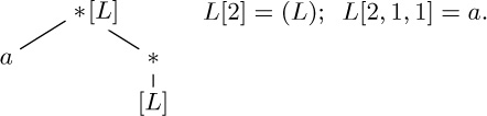
20. (Intuitively, the correspondence between 0-2-trees and binary trees is obtained by removing all terminal nodes of the 0-2-tree; see the important construction in Section 2.3.4.5.) Let a 0-2-tree with one node correspond to the empty binary tree; and let a 0-2-tree with more than one node, consisting therefore of a root r and 0-2-trees $T_{1}$ and $T_{2}$, correspond to the binary tree with root r, left subtree $T'_{1}$, and right subtree $T'_{2}$, where $T_{1}$ and $T_{2}$ correspond respectively to $T'_{1}$ and $T'_{2}$.
21. $1+0·n_{1}+1·n_{2}+\cdots+(m-1)·n_{m}$. Proof: The number of nodes in the tree is $n_{0}+n_{1}+n_{2}+\cdots+n_{m}$, and this also equals 1 + (number of children in the tree) = $1+0·n_{0}+1·n_{1}+2·n_{2}+\cdots+m·n_{m}$.
22. The basic idea is to proceed recursively, with the representation of a nonempty binary tree defined to be the representation of its root plus half-size-and-rotated representations of its left and right subtrees. Thus an arbitrarily large binary tree can be represented on a single sheet of paper, if one has a sufficiently powerful magnifying glass.
Many variations on this theme are possible. For example, one idea is to represent the root by a line from the center of a given landscape-oriented page to the top edge, and to rotate the left-subtree representation by $90^{°}$ clockwise in the left halfpage, the right-subtree representation by $90^{°}$ counterclockwise in the right halfpage. Each node is then represented by a line. (When this method is applied to a complete binary tree having $2^{k}-1$ nodes on k levels, it yields so-called “H-trees,” which are the most efficient layouts of such binary trees on a VLSI chip; see R. P. Brent and H. T. Kung, Inf. Proc. Letters 11 (1980), 46–48.)

Another idea is to represent an empty binary tree by some sort of box, and to rotate the subtree representations of nonempty binary trees so that left subsubtrees are alternately to the left of or below the corresponding right subsubtrees, depending on whether the depth of recursion is even or odd. Then the boxes correspond to external nodes in an extended binary tree (see Section 2.3.4.5). This representation, which is strongly related to the 2-d trees and quadtrees discussed in Section 6.5, is especially appropriate when the external nodes carry information but the internal nodes do not.