Many persons who are not conversant with mathematical studies
imagine that because the business of [Babbage’s Analytical Engine] is to
give its results in numerical notation, the nature of its processes must
consequently be arithmetical and numerical, rather than algebraical and
analytical. This is an error. The engine can arrange and combine its
numerical quantities exactly as if they were letters or any other general
symbols; and in fact it might bring out its results in algebraical notation,
were provisions made accordingly.
— AUGUSTA ADA, Countess of Lovelace (1843)
Practice yourself, for heaven’s sake, in little things;
and thence proceed to greater.
— EPICTETUS (Discourses IV.i)
The notion of an algorithm is basic to all of computer programming, so we should begin with a careful analysis of this concept.
The word “algorithm” itself is quite interesting; at first glance it may look as though someone intended to write “logarithm” but jumbled up the first four letters. The word did not appear in Webster’s New World Dictionary as late as 1957; we find only the older form “algorism” with its ancient meaning, the process of doing arithmetic using Arabic numerals. During the Middle Ages, abacists computed on the abacus and algorists computed by algorism. By the time of the Renaissance, the origin of this word was in doubt, and early linguists attempted to guess at its derivation by making combinations like algiros [painful]+arithmos [number]; others said no, the word comes from “King Algor of Castile.” Finally, historians of mathematics found the true origin of the word algorism: It comes from the name of a famous Persian textbook author, Abū ‘Abd Allāh Muh. ammad ibn Mūsā al-Khwārizmī (c. 825) — literally, “Father of Abdullah, Mohammed, son of Moses, native of Khwārizm.” The Aral Sea in Central Asia was once known as Lake Khwārizm, and the Khwārizm region is located in the Amu River basin just south of that sea. Al-Khwārizmī wrote the celebrated Arabic text Kitāb al-jabr wa’l-muqābala (“Rules of restoring and equating”); another word, “algebra,” stems from the title of that book, which was a systematic study of the solution of linear and quadratic equations. [For notes on al-Khwārizmī’s life and work, see H. Zemanek, Lecture Notes in Computer Science 122 (1981), 1–81.]
Gradually the form and meaning of algorism became corrupted; as explained by the Oxford English Dictionary, the word “passed through many pseudo-etymological perversions, including a recent algorithm, in which it is learnedly confused” with the Greek root of the word arithmetic. This change from “algorism” to “algorithm” is not hard to understand in view of the fact that people had forgotten the original derivation of the word. An early German mathematical dictionary, Vollständiges mathematisches Lexicon (Leipzig: 1747), gave the following definition for the word Algorithmus: “Under this designation are combined the notions of the four types of arithmetic calculations, namely addition, multiplication, subtraction, and division.” The Latin phrase algorithmus infinitesimalis was at that time used to denote “ways of calculation with infinitely small quantities, as invented by Leibniz.”
By 1950, the word algorithm was most frequently associated with Euclid’s algorithm, a process for finding the greatest common divisor of two numbers that appears in Euclid’s Elements (Book 7, Propositions 1 and 2). It will be instructive to exhibit Euclid’s algorithm here:
Algorithm E (Euclid’s algorithm). Given two positive integers m and n, find their greatest common divisor, that is, the largest positive integer that evenly divides both m and n.
E1. [Find remainder.] Divide m by n and let r be the remainder. (We will have 0 ≤ r < n.)
E2. [Is it zero?] If r = 0, the algorithm terminates; n is the answer.
E3. [Reduce.] Set $m←n$, $n←r$, and go back to step E1. 
Of course, Euclid did not present his algorithm in just this manner. The format above illustrates the style in which all of the algorithms throughout this book will be presented.
Each algorithm we consider has been given an identifying letter (E in the preceding example), and the steps of the algorithm are identified by this letter followed by a number (E1, E2, E3). The chapters are divided into numbered sections; within a section the algorithms are designated by letter only, but when algorithms are referred to in other sections, the appropriate section number is attached. For example, we are now in Section 1.1; within this section Euclid’s algorithm is called Algorithm E, while in later sections it is referred to as Algorithm 1.1E.
Each step of an algorithm, such as step E1 above, begins with a phrase in brackets that sums up as briefly as possible the principal content of that step. This phrase also usually appears in an accompanying flow chart, such as Fig. 1, so that the reader will be able to picture the algorithm more readily.
After the summarizing phrase comes a description in words and symbols of some action to be performed or some decision to be made. Parenthesized comments, like the second sentence in step E1, may also appear. Comments are included as explanatory information about that step, often indicating certain invariant characteristics of the variables or the current goals. They do not specify actions that belong to the algorithm, but are meant only for the reader’s benefit as possible aids to comprehension.
The arrow “←” in step E3 is the all-important replacement operation, sometimes called assignment or substitution: “$m←n$” means that the value of variable m is to be replaced by the current value of variable n. When Algorithm E begins, the values of m and n are the originally given numbers; but when it ends, those variables will have, in general, different values. An arrow is used to distinguish the replacement operation from the equality relation: We will not say, “Set m = n,” but we will perhaps ask, “Does m = n?” The “=” sign denotes a condition that can be tested, the “←” sign denotes an action that can be performed. The operation of increasing n by one is denoted by “$n←n+1$” (read “n is replaced by n + 1” or “n gets n + 1”). In general, “variable ← formula” means that the formula is to be computed using the present values of any variables appearing within it; then the result should replace the previous value of the variable at the left of the arrow. Persons untrained in computer work sometimes have a tendency to say “n becomes n + 1” and to write “$n→n+1$” for the operation of increasing n by one; this symbolism can only lead to confusion because of its conflict with standard conventions, and it should be avoided.
Notice that the order of actions in step E3 is important: “Set $m←n$, $n←r$” is quite different from “Set $n←r$, $m←n$,” since the latter would imply that the previous value of n is lost before it can be used to set m. Thus the latter sequence is equivalent to “Set $n←r$, $m←r$.” When several variables are all to be set equal to the same quantity, we can use multiple arrows; for example, “$n←r$, $m←r$” may be written “$n←m←r$.” To interchange the values of two variables, we can write “Exchange $m↔n$”; this action could also be specified by using a new variable t and writing “Set $t←m$, $m←n$, $n←t$.”
An algorithm starts at the lowest-numbered step, usually step 1, and it performs subsequent steps in sequential order unless otherwise specified. In step E3, the imperative “go back to step E1” specifies the computational order in an obvious fashion. In step E2, the action is prefaced by the condition “If r = 0”; so if r ≠ 0, the rest of that sentence does not apply and no action is specified. We might have added the redundant sentence, “If r ≠ 0, go on to step E3.”
The heavy vertical line “” appearing at the end of step E3 is used to indicate the end of an algorithm and the resumption of text.
We have now discussed virtually all the notational conventions used in the algorithms of this book, except for a notation used to denote “subscripted” or “indexed” items that are elements of an ordered array. Suppose we have n quantities, $v_{1},v_{2},...,v_{n}$; instead of writing $v_{j}$ for the j th element, the notation $v[j]$ is often used. Similarly, $a[i,j]$ is sometimes used in preference to a doubly subscripted notation like $a_{ij}$. Sometimes multiple-letter names are used for variables, usually set in capital letters; thus TEMP might be the name of a variable used for temporarily holding a computed value, PRIME[K] might denote the Kth prime number, and so on.
So much for the form of algorithms; now let us perform one. It should be mentioned immediately that the reader should not expect to read an algorithm as if it were part of a novel; such an attempt would make it pretty difficult to understand what is going on. An algorithm must be seen to be believed, and the best way to learn what an algorithm is all about is to try it. The reader should always take pencil and paper and work through an example of each algorithm immediately upon encountering it in the text. Usually the outline of a worked example will be given, or else the reader can easily conjure one up. This is a simple and painless way to gain an understanding of a given algorithm, and all other approaches are generally unsuccessful.
Let us therefore work out an example of Algorithm E. Suppose that we are given m = 119 and n = 544; we are ready to begin, at step E1. (The reader should now follow the algorithm as we give a play-by-play account.) Dividing m by n in this case is quite simple, almost too simple, since the quotient is zero and the remainder is 119. Thus, $r←119$. We proceed to step E2, and since r ≠ 0 no action occurs. In step E3 we set $m←544$, $n←119$. It is clear that if m < n originally, the quotient in step E1 will always be zero and the algorithm will always proceed to interchange m and n in this rather cumbersome fashion. We could insert a new step at the beginning:
E0. [Ensure m ≥ n.] If m < n, exchange m ↔ n.
This would make no essential change in the algorithm, except to increase its length slightly, and to decrease its running time in about one half of all cases.
Back at step E1, we find that $544/119=4+68/119$, so $r←68$. Again E2 is inapplicable, and at E3 we set $m←119$, $n←68$. The next round sets $r←51$, and ultimately $m←68$, $n←51$. Next $r←17$, and $m←51$, $n←17$. Finally, when 51 is divided by 17, we set $r←0$, so at step E2 the algorithm terminates. The greatest common divisor of 119 and 544 is 17.
So this is an algorithm. The modern meaning for algorithm is quite similar to that of recipe, process, method, technique, procedure, routine, rigmarole, except that the word “algorithm” connotes something just a little different. Besides merely being a finite set of rules that gives a sequence of operations for solving a specific type of problem, an algorithm has five important features:
1) Finiteness. An algorithm must always terminate after a finite number of steps. Algorithm E satisfies this condition, because after step E1 the value of r is less than n; so if r ≠ 0, the value of n decreases the next time step E1 is encountered. A decreasing sequence of positive integers must eventually terminate, so step E1 is executed only a finite number of times for any given original value of n. Note, however, that the number of steps can become arbitrarily large; certain huge choices of m and n will cause step E1 to be executed more than a million times.
(A procedure that has all of the characteristics of an algorithm except that it possibly lacks finiteness may be called a computational method. Euclid originally presented not only an algorithm for the greatest common divisor of numbers, but also a very similar geometrical construction for the “greatest common measure” of the lengths of two line segments; this is a computational method that does not terminate if the given lengths are incommensurable. Another example of a nonterminating computational method is a reactive process, which continually interacts with its environment.)
2) Definiteness. Each step of an algorithm must be precisely defined; the actions to be carried out must be rigorously and unambiguously specified for each case. The algorithms of this book will hopefully meet this criterion, but they are specified in the English language, so there is a possibility that the reader might not understand exactly what the author intended. To get around this difficulty, formally defined programming languages or computer languages are designed for specifying algorithms, in which every statement has a very definite meaning. Many of the algorithms of this book will be given both in English and in a computer language. An expression of a computational method in a computer language is called a program.
In Algorithm E, the criterion of definiteness as applied to step E1 means that the reader is supposed to understand exactly what it means to divide m by n and what the remainder is. In actual fact, there is no universal agreement about what this means if m and n are not positive integers; what is the remainder of −8 divided by −π? What is the remainder of $59/13$ divided by zero? Therefore the criterion of definiteness means we must make sure that the values of m and n are always positive integers whenever step E1 is to be executed. This is initially true, by hypothesis; and after step E1, r is a nonnegative integer that must be nonzero if we get to step E3. So m and n are indeed positive integers as required.
3) Input. An algorithm has zero or more inputs: quantities that are given to it initially before the algorithm begins, or dynamically as the algorithm runs. These inputs are taken from specified sets of objects. In Algorithm E, for example, there are two inputs, namely m and n, both taken from the set of positive integers.
4) Output. An algorithm has one or more outputs: quantities that have a specified relation to the inputs. Algorithm E has one output, namely n in step E2, the greatest common divisor of the two inputs.
(We can easily prove that this number is indeed the greatest common divisor, as follows. After step E1, we have
$m=qn+r$,
for some integer q. If r = 0, then m is a multiple of n, and clearly in such a case n is the greatest common divisor of m and n. If r ≠ 0, note that any number that divides both m and n must divide $m-qn=r$, and any number that divides both n and r must divide $qn+r=m$; so the set of common divisors of m and n is the same as the set of common divisors of n and r. In particular, the greatest common divisor of m and n is the same as the greatest common divisor of n and r. Therefore step E3 does not change the answer to the original problem.)
5) Effectiveness. An algorithm is also generally expected to be effective, in the sense that its operations must all be sufficiently basic that they can in principle be done exactly and in a finite length of time by someone using pencil and paper. Algorithm E uses only the operations of dividing one positive integer by another, testing if an integer is zero, and setting the value of one variable equal to the value of another. These operations are effective, because integers can be represented on paper in a finite manner, and because there is at least one method (the “division algorithm”) for dividing one by another. But the same operations would not be effective if the values involved were arbitrary real numbers specified by an infinite decimal expansion, nor if the values were the lengths of physical line segments (which cannot be specified exactly). Another example of a noneffective step is, “If 4 is the largest integer n for which there is a solution to the equation $w^{n}+x^{n}+y^{n}=z^{n}$ in positive integers w, x, y, and z, then go to step E4.” Such a statement would not be an effective operation until someone successfully constructs an algorithm to determine whether 4 is or is not the largest integer with the stated property.
Let us try to compare the concept of an algorithm with that of a cookbook recipe. A recipe presumably has the qualities of finiteness (although it is said that a watched pot never boils), input (eggs, flour, etc.), and output (TV dinner, etc.), but it notoriously lacks definiteness. There are frequent cases in which a cook’s instructions are indefinite: “Add a dash of salt.” A “dash” is defined to be “less than ⅛ teaspoon,” and salt is perhaps well enough defined; but where should the salt be added — on top? on the side? Instructions like “toss lightly until mixture is crumbly” or “warm cognac in small saucepan” are quite adequate as explanations to a trained chef, but an algorithm must be specified to such a degree that even a computer can follow the directions. Nevertheless, a computer programmer can learn much by studying a good recipe book. (The author has in fact barely resisted the temptation to name the present volume “The Programmer’s Cookbook.” Perhaps someday he will attempt a book called “Algorithms for the Kitchen.”)
We should remark that the finiteness restriction is not really strong enough for practical use. A useful algorithm should require not only a finite number of steps, but a very finite number, a reasonable number. For example, there is an algorithm that determines whether or not the game of chess can always be won by White if no mistakes are made (see exercise 2.2.3–28). That algorithm can solve a problem of intense interest to thousands of people, yet it is a safe bet that we will never in our lifetimes know the answer; the algorithm requires fantastically large amounts of time for its execution, even though it is finite. See also Chapter 8 for a discussion of some finite numbers that are so large as to actually be beyond comprehension.
In practice we not only want algorithms, we want algorithms that are good in some loosely defined aesthetic sense. One criterion of goodness is the length of time taken to perform the algorithm; this can be expressed in terms of the number of times each step is executed. Other criteria are the adaptability of the algorithm to different kinds of computers, its simplicity and elegance, etc.
We often are faced with several algorithms for the same problem, and we must decide which is best. This leads us to the extremely interesting and all-important field of algorithmic analysis: Given an algorithm, we want to determine its performance characteristics.
For example, let’s consider Euclid’s algorithm from this point of view. Suppose we ask the question, “Assuming that the value of n is known but m is allowed to range over all positive integers, what is the average number of times, $T_{n}$, that step E1 of Algorithm E will be performed?” In the first place, we need to check that this question does have a meaningful answer, since we are trying to take an average over infinitely many choices for m. But it is evident that after the first execution of step E1 only the remainder of m after division by n is relevant. So all we must do to find $T_{n}$ is to try the algorithm for $m=1,m=2,...,m=n$, count the total number of times step E1 has been executed, and divide by n.
Now the important question is to determine the nature of $T_{n}$; is it approximately equal to ${\frac{1}{3}}n$, or $\sqrt{n}$, for instance? As a matter of fact, the answer to this question is an extremely difficult and fascinating mathematical problem, not yet completely resolved, which is examined in more detail in Section 4.5.3. For large values of n it is possible to prove that $T_{n}$ is approximately $(12(\ln 2)/π^{2})\ln n$, that is, proportional to the natural logarithm of n, with a constant of proportionality that might not have been guessed offhand! For further details about Euclid’s algorithm, and other ways to calculate the greatest common divisor, see Section 4.5.2.
Analysis of algorithms is the name the author likes to use to describe investigations such as this. The general idea is to take a particular algorithm and to determine its quantitative behavior; occasionally we also study whether or not an algorithm is optimal in some sense. The theory of algorithms is another subject entirely, dealing primarily with the existence or nonexistence of effective algorithms to compute particular quantities.
So far our discussion of algorithms has been rather imprecise, and a mathematically oriented reader is justified in thinking that the preceding commentary makes a very shaky foundation on which to erect any theory about algorithms. We therefore close this section with a brief indication of one method by which the concept of algorithm can be firmly grounded in terms of mathematical set theory. Let us formally define a computational method to be a quadruple (Q, I, Ω, f), in which Q is a set containing subsets I and Ω, and f is a function from Q into itself. Furthermore f should leave Ω pointwise fixed; that is, $f(q)$ should equal q for all elements q of Ω. The four quantities Q, I, Ω, f are intended to represent respectively the states of the computation, the input, the output, and the computational rule. Each input x in the set I defines a computational sequence, $x_{0},x_{1},x_{2},...$, as follows:

The computational sequence is said to terminate in k steps if k is the smallest integer for which $x_{k}$ is in Ω, and in this case it is said to produce the output $x_{k}$ from x. (Notice that if $x_{k}$ is in Ω, so is $x_{k+1}$, because $x_{k+1}=x_{k}$ in such a case.) Some computational sequences may never terminate; an algorithm is a computational method that terminates in finitely many steps for all x in I.
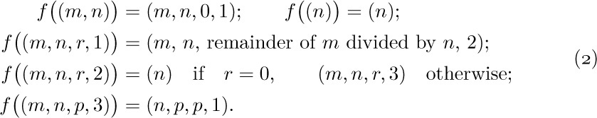
Algorithm E may, for example, be formalized in these terms as follows: Let Q be the set of all singletons $(n)$, all ordered pairs $(m,n)$, and all ordered quadruples $(m,n,r,1)$, $(m,n,r,2)$, and $(m,n,p,3)$, where m, n, and p are positive integers and r is a nonnegative integer. Let I be the subset of all pairs $(m,n)$ and let Ω be the subset of all singletons $(n)$. Let f be defined as follows:
The correspondence between this notation and Algorithm E is evident.
This formulation of the concept of an algorithm does not include the restriction of effectiveness mentioned earlier. For example, Q might denote infinite sequences that are not computable by pencil and paper methods, or f might involve operations that mere mortals cannot always perform. If we wish to restrict the notion of algorithm so that only elementary operations are involved, we can place restrictions on Q, I, Ω, and f, for example as follows: Let A be a finite set of letters, and let $A^{*}$ be the set of all strings on A (the set of all ordered sequences $x_{1}x_{2}...x_{n}$, where n ≥ 0 and $x_{j}$ is in A for 1 ≤ j ≤ n). The idea is to encode the states of the computation so that they are represented by strings of $A^{*}$. Now let N be a nonnegative integer and let Q be the set of all $(σ,j)$, where σ is in $A^{*}$ and j is an integer, 0 ≤ j ≤ N; let I be the subset of Q with j = 0 and let Ω be the subset with j = N. If θ and σ are strings in $A^{*}$, we say that θ occurs in σ if σ has the form $αθω$ for strings α and ω. To complete our definition, let f be a function of the following type, defined by the strings $θ_{j}$, $φ_{j}$ and the integers $a_{j}$, $b_{j}$ for 0 ≤ j < N:
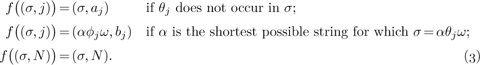
Every step of such a computational method is clearly effective, and experience shows that pattern-matching rules of this kind are also powerful enough to do anything we can do by hand. There are many other essentially equivalent ways to formulate the concept of an effective computational method (for example, using Turing machines). The formulation above is virtually the same as that given by A. A. Markov in his book The Theory of Algorithms [Trudy Mat. Inst. Akad. Nauk 42 (1954), 1–376], later revised and enlarged by N. M. Nagorny (Moscow: Nauka, 1984; English edition, Dordrecht: Kluwer, 1988).
Exercises
1. [10] The text showed how to interchange the values of variables m and n, using the replacement notation, by setting $t←m$, $m←n$, $n←t$. Show how the values of four variables $(a,b,c,d)$ can be rearranged to $(b,c,d,a)$ by a sequence of replacements. In other words, the new value of a is to be the original value of b, etc. Try to use the minimum number of replacements.
2. [15] Prove that m is always greater than n at the beginning of step E1, except possibly the first time this step occurs.
3. [20] Change Algorithm E (for the sake of efficiency) so that all trivial replacement operations such as “$m←n$” are avoided. Write this new algorithm in the style of Algorithm E, and call it Algorithm F.
4. [16] What is the greatest common divisor of 2166 and 6099?
![]() 5. [12] Show that the “Procedure for Reading This Set of Books” that appears after the preface actually fails to be a genuine algorithm on at least three of our five counts! Also mention some differences in format between it and Algorithm E.
5. [12] Show that the “Procedure for Reading This Set of Books” that appears after the preface actually fails to be a genuine algorithm on at least three of our five counts! Also mention some differences in format between it and Algorithm E.
6. [20] What is $T_{5}$, the average number of times step E1 is performed when n = 5?
![]() 7. [M21] Suppose that m is known and n is allowed to range over all positive integers; let $U_{m}$ be the average number of times that step E1 is executed in Algorithm E. Show that $U_{m}$ is well defined. Is $U_{m}$ in any way related to $T_{m}$?
7. [M21] Suppose that m is known and n is allowed to range over all positive integers; let $U_{m}$ be the average number of times that step E1 is executed in Algorithm E. Show that $U_{m}$ is well defined. Is $U_{m}$ in any way related to $T_{m}$?
8. [M25] Give an “effective” formal algorithm for computing the greatest common divisor of positive integers m and n, by specifying $θ_{j}$, $φ_{j}$, $a_{j}$, $b_{j}$ as in Eqs. (3). Let the input be represented by the string $a^{m}b^{n}$, that is, m a’s followed by n b’s. Try to make your solution as simple as possible. [Hint: Use Algorithm E, but instead of division in step E1, set $r←|m-n|$, $n←\min(m,n)$.]
![]() 9. [M30] Suppose that $C_{1}=(Q_{1},I_{1},Ω_{1},f_{1})$ and $C_{2}=(Q_{2},I_{2},Ω_{2},f_{2})$ are computational methods. For example, $C_{1}$ might stand for Algorithm E as in Eqs. (2), except that m and n are restricted in magnitude, and $C_{2}$ might stand for a computer program implementation of Algorithm E. (Thus $Q_{2}$ might be the set of all states of the machine, i.e., all possible configurations of its memory and registers; $f_{2}$ might be the definition of single machine actions; and $I_{2}$ might be the set of initial states, each including the program that determines the greatest common divisor as well as the particular values of m and n.)
9. [M30] Suppose that $C_{1}=(Q_{1},I_{1},Ω_{1},f_{1})$ and $C_{2}=(Q_{2},I_{2},Ω_{2},f_{2})$ are computational methods. For example, $C_{1}$ might stand for Algorithm E as in Eqs. (2), except that m and n are restricted in magnitude, and $C_{2}$ might stand for a computer program implementation of Algorithm E. (Thus $Q_{2}$ might be the set of all states of the machine, i.e., all possible configurations of its memory and registers; $f_{2}$ might be the definition of single machine actions; and $I_{2}$ might be the set of initial states, each including the program that determines the greatest common divisor as well as the particular values of m and n.)
Formulate a set-theoretic definition for the concept “$C_{2}$ is a representation of $C_{1}$” or “$C_{2}$ simulates $C_{1}$.” This is to mean intuitively that any computation sequence of $C_{1}$ is mimicked by $C_{2}$, except that $C_{2}$ might take more steps in which to do the computation and it might retain more information in its states. (We thereby obtain a rigorous interpretation of the statement, “Program X is an implementation of Algorithm Y.”)
In this section we shall investigate the mathematical notations that occur throughout The Art of Computer Programming, and we’ll derive several basic formulas that will be used repeatedly. Even a reader not concerned with the more complex mathematical derivations should at least become familiar with the meanings of the various formulas, so as to be able to use the results of the derivations.
Mathematical notation is used for two main purposes in this book: to describe portions of an algorithm, and to analyze the performance characteristics of an algorithm. The notation used in descriptions of algorithms is quite simple, as explained in the previous section. When analyzing the performance of algorithms, we need to use other more specialized notations.
Most of the algorithms we will discuss are accompanied by mathematical calculations that determine the speed at which the algorithm may be expected to run. These calculations draw on nearly every branch of mathematics, and a separate book would be necessary to develop all of the mathematical concepts that are used in one place or another. However, the majority of the calculations can be carried out with a knowledge of college algebra, and the reader with a knowledge of elementary calculus will be able to understand nearly all of the mathematics that appears. Sometimes we will need to use deeper results of complex variable theory, group theory, number theory, probability theory, etc.; in such cases the topic will be explained in an elementary manner, if possible, or a reference to other sources of information will be given.
The mathematical techniques involved in the analysis of algorithms usually have a distinctive flavor. For example, we will quite often find ourselves working with finite summations of rational numbers, or with the solutions to recurrence relations. Such topics are traditionally given only a light treatment in mathematics courses, and so the following subsections are designed not only to give a thorough drilling in the use of the notations to be defined but also to illustrate in depth the types of calculations and techniques that will be most useful to us.
Important note: Although the following subsections provide a rather extensive training in the mathematical skills needed in connection with the study of computer algorithms, most readers will not see at first any very strong connections between this material and computer programming (except in Section 1.2.1). The reader may choose to read the following subsections carefully, with implicit faith in the author’s assertion that the topics treated here are indeed very relevant; but it is probably preferable, for motivation, to skim over this section lightly at first, and (after seeing numerous applications of the techniques in future chapters) return to it later for more intensive study. If too much time is spent studying this material when first reading the book, a person might never get on to the computer programming topics! However, each reader should at least become familiar with the general contents of these subsections, and should try to solve a few of the exercises, even on first reading. Section 1.2.10 should receive particular attention, since it is the point of departure for most of the theoretical material developed later. Section 1.3, which follows 1.2, abruptly leaves the realm of “pure mathematics” and enters into “pure computer programming.”
An expansion and more leisurely presentation of much of the following material can be found in the book Concrete Mathematics by Graham, Knuth, and Patashnik, second edition (Reading, Mass.: Addison–Wesley, 1994). That book will be called simply CMath when we need to refer to it later.
Let $P(n)$ be some statement about the integer n; for example, $P(n)$ might be “n times $(n+3)$ is an even number,” or “if n ≥ 10, then $2^{n}\gt n^{3}$.” Suppose we want to prove that $P(n)$ is true for all positive integers n. An important way to do this is:
a) Give a proof that $P(1)$ is true.
b) Give a proof that “if all of $P(1),P(2),...,P(n)$ are true, then $P(n+1)$ is also true”; this proof should be valid for any positive integer n.
As an example, consider the following series of equations, which many people have discovered independently since ancient times:
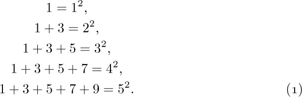
We can formulate the general property as follows:

Let us, for the moment, call this equation $P(n)$; we wish to prove that $P(n)$ is true for all positive n. Following the procedure outlined above, we have:
a) “$P(1)$ is true, since $1=1^{2}$.”
b) “If all of $P(1),...,P(n)$ are true, then, in particular, $P(n)$ is true, so Eq. (2) holds; adding 2n + 1 to both sides we obtain
$1+3+···+(2n-1)+(2n+1)=n^{2}+2n+1=(n+1)^{2}$,
which proves that $P(n+1)$ is also true.”
We can regard this method as an algorithmic proof procedure. In fact, the following algorithm produces a proof of $P(n)$ for any positive integer n, assuming that steps (a) and (b) above have been worked out:
Algorithm I (Construct a proof). Given a positive integer n, this algorithm will output a proof that $P(n)$ is true.
I1. [Prove $P(1)$.] Set $k←1$, and, according to (a), output a proof of $P(1)$.
I2. [k = n?] If k = n, terminate the algorithm; the required proof has been output.
I3. [Prove $P(k+1)$.] According to (b), output a proof that “If all of $P(1),...,P(k)$ are true, then $P(k+1)$ is true.” Also output “We have already proved $P(1),...,P(k)$; hence $P(k+1)$ is true.”
I4. [Increase k.] Increase k by 1 and go to step I2.
Since this algorithm clearly presents a proof of $P(n)$, for any given n, the proof technique consisting of steps (a) and (b) is logically valid. It is called proof by mathematical induction.
The concept of mathematical induction should be distinguished from what is usually called inductive reasoning in science. A scientist takes specific observations and creates, by “induction,” a general theory or hypothesis that accounts for these facts; for example, we might observe the five relations in (1), above, and formulate (2). In this sense, induction is no more than our best guess about the situation; mathematicians would call it an empirical result or a conjecture.
Another example will be helpful. Let $p(n)$ denote the number of partitions of n, that is, the number of different ways to write n as a sum of positive integers, disregarding order. Since 5 can be partitioned in exactly seven ways,
1 + 1 + 1 + 1 + 1 = 2 + 1 + 1 + 1 = 2 + 2 + 1 = 3 + 1 + 1 = 3 + 2 = 4 + 1 = 5,
we have $p(5)=7$. In fact, it is easy to establish the first few values,
$p(1)=1$, $p(2)=2$, $p(3)=3$, $p(4)=5$, $p(5)=7$.
At this point we might tentatively formulate, by induction, the hypothesis that the sequence $p(2),p(3),...$ runs through the prime numbers. To test this hypothesis, we proceed to calculate $p(6)$ and behold! $p(6)=11$, confirming our conjecture.
[Unfortunately, $p(7)$ turns out to be 15, spoiling everything, and we must try again. The numbers $p(n)$ are known to be quite complicated, although S. Ramanujan succeeded in guessing and proving many remarkable things about them. For further information, see G. H. Hardy, Ramanujan (London: Cambridge University Press, 1940), Chapters 6 and 8. See also Section 7.2.1.4.]
Mathematical induction is quite different from induction in the sense just explained. It is not just guesswork, but a conclusive proof of a statement; indeed, it is a proof of infinitely many statements, one for each n. It has been called “induction” only because one must first decide somehow what is to be proved, before one can apply the technique of mathematical induction. Henceforth in this book we shall use the word induction only when we wish to imply proof by mathematical induction.
There is a geometrical way to prove Eq. (2). Figure 3 shows, for n = 6, $n^{2}$ cells broken into groups of $1+3+···+(2n-1)$ cells. However, in the final analysis, this picture can be regarded as a “proof” only if we show that the construction can be carried out for all n, and such a demonstration is essentially the same as a proof by induction.
Our proof of Eq. (2) used only a special case of (b); we merely showed that the truth of $P(n)$ implies the truth of $P(n+1)$. This is an important simple case that arises frequently, but our next example illustrates the power of the method a little more. We define the Fibonacci sequence $F_{0},F_{1},F_{2},...$ by the rule that $F_{0}=0$, $F_{1}=1$, and every further term is the sum of the preceding two. Thus the sequence begins 0, 1, 1, 2, 3, 5, 8, 13, ...; we will investigate it in detail in Section 1.2.8. We will now prove that if φ is the number $(1+\sqrt{5})/2$ we have

for all positive integers n. Call this formula $P(n)$.
If n = 1, then $F_{1}=1=φ^{0}=φ^{1-1}$, so step (a) has been done. For step (b) we notice first that $P(2)$ is also true, since $F_{2}=1\lt 1.6\lt φ^{1}=φ^{2-1}$. Now, if all of $P(1),P(2),...,P(n)$ are true and n > 1, we know in particular that $P(n-1)$ and $P(n)$ are true; so $F_{n-1}≤φ^{n-2}$ and $F_{n}≤φ^{n-1}$. Adding these inequalities, we get

The important property of the number φ, indeed the reason we chose this number for this problem in the first place, is that

Plugging (5) into (4) gives $F_{n+1}≤φ^{n}$, which is $P(n+1)$. So step (b) has been done, and (3) has been proved by mathematical induction. Notice that we approached step (b) in two different ways here: We proved $P(n+1)$ directly when n = 1, and we used an inductive method when n > 1. This was necessary, since when n = 1 our reference to $P(n-1)=P(0)$ would not have been legitimate.
Mathematical induction can also be used to prove things about algorithms. Consider the following generalization of Euclid’s algorithm.
Algorithm E (Extended Euclid’s algorithm). Given two positive integers m and n, we compute their greatest common divisor d, and we also compute two not-necessarily-positive integers a and b such that $am+bn=d$.
E1. [Initialize.] Set $a'←b←1$, $a←b'←0$, $c←m$, $d←n$.
E2. [Divide.] Let q and r be the quotient and remainder, respectively, of c divided by d. (We have $c=qd+r$ and 0 ≤ r < d.)
E3. [Remainder zero?] If r = 0, the algorithm terminates; we have in this case $am+bn=d$ as desired.
E4. [Recycle.] Set $c←d$, $d←r$, $t←a'$, $a'←a$, $a←t-qa$, $t←b'$, $b'←b$, $b←t-qb$, and go back to E2.
If we suppress the variables a, b, a′, and b′ from this algorithm and use m and n for the auxiliary variables c and d, we have our old algorithm, 1.1E. The new version does a little more, by determining the coefficients a and b. Suppose that m = 1769 and n = 551; we have successively (after step E2):

The answer is correct: $5×1769-16×551=8845-8816=29$, the greatest common divisor of 1769 and 551.
The problem is to prove that this algorithm works properly, for all m and n. We can try to apply the method of mathematical induction by letting $P(n)$ be the statement “Algorithm E works for n and all integers m.” However, that approach doesn’t work out so easily, and we need to prove some extra facts. After a little study, we find that something must be proved about a, b, a′, and b′, and the appropriate fact is that the equalities

always hold whenever step E2 is executed. We may prove these equalities directly by observing that they are certainly true the first time we get to E2, and that step E4 does not change their validity. (See exercise 6.)
Now we are ready to show that Algorithm E is valid, by induction on n: If m is a multiple of n, the algorithm obviously works properly, since we are done immediately at E3 the first time. This case always occurs when n = 1. The only case remaining is when n > 1 and m is not a multiple of n. In such a case, the algorithm proceeds to set $c←n$, $d←r$ after the first execution, and since r < n, we may assume by induction that the final value of d is the gcd of n and r. By the argument given in Section 1.1, the pairs $\{m,n\}$ and $\{n,r\}$ have the same common divisors, and, in particular, they have the same greatest common divisor. Hence d is the gcd of m and n, and $am+bn=d$ by (6).
The italicized phrase in the proof above illustrates the conventional language that is so often used in an inductive proof: When doing part (b) of the construction, rather than saying “We will now assume $P(1),P(2),...,P(n)$, and with this assumption we will prove $P(n+1)$,” we often say simply “We will now prove $P(n)$; we may assume by induction that $P(k)$ is true whenever 1 ≤ k < n.”
If we examine this argument very closely and change our viewpoint slightly, we can envision a general method applicable to proving the validity of any algorithm. The idea is to take a flow chart for some algorithm and to label each of the arrows with an assertion about the current state of affairs at the time the computation traverses that arrow. See Fig. 4, where the assertions have been labeled A1, A2, ..., A6. (All of these assertions have the additional stipulation that the variables are integers; this stipulation has been omitted to save space.) A1 gives the initial assumptions upon entry to the algorithm, and A4 states what we hope to prove about the output values a, b, and d.

Fig. 4. Flow chart for Algorithm E, labeled with assertions that prove the validity of the algorithm.
The general method consists of proving, for each box in the flow chart, that

Thus, for example, we must prove that either A2 or A6 before E2 implies A3 after E2. (In this case A2 is a stronger statement than A6; that is, A2 implies A6. So we need only prove that A6 before E2 implies A3 after. Notice that the condition d > 0 is necessary in A6 just to prove that operation E2 even makes sense.) It is also necessary to show that A3 and r = 0 implies A4; that A3 and r ≠ 0 implies A5; etc. Each of the required proofs is very straightforward.
Once statement (7) has been proved for each box, it follows that all assertions are true during any execution of the algorithm. For we can now use induction on the number of steps of the computation, in the sense of the number of arrows traversed in the flow chart. While traversing the first arrow, the one leading from “Start”, the assertion A1 is true since we always assume that our input values meet the specifications; so the assertion on the first arrow traversed is correct. If the assertion that labels the nth arrow is true, then by (7) the assertion that labels the (n + 1)st arrow is also true.
Using this general method, the problem of proving that a given algorithm is valid evidently consists mostly of inventing the right assertions to put in the flow chart. Once this inductive leap has been made, it is pretty much routine to carry out the proofs that each assertion leading into a box logically implies each assertion leading out. In fact, it is pretty much routine to invent the assertions themselves, once a few of the difficult ones have been discovered; thus it is very simple in our example to write out essentially what A2, A3, and A5 must be, if only A1, A4, and A6 are given. In our example, assertion A6 is the creative part of the proof; all the rest could, in principle, be supplied mechanically. Hence no attempt has been made to give detailed formal proofs of the algorithms that follow in this book, at the level of detail found in Fig. 4. It suffices to state the key inductive assertions. Those assertions either appear in the discussion following an algorithm or they are given as parenthetical remarks in the text of the algorithm itself.
This approach to proving the correctness of algorithms has another aspect that is even more important: It mirrors the way we understand an algorithm. Recall that in Section 1.1 the reader was cautioned not to expect to read an algorithm like part of a novel; one or two trials of the algorithm on some sample data were recommended. This was done expressly because an example runthrough of the algorithm helps a person formulate the various assertions mentally. It is the contention of the author that we really understand why an algorithm is valid only when we reach the point that our minds have implicitly filled in all the assertions, as was done in Fig. 4. This point of view has important psychological consequences for the proper communication of algorithms from one person to another: It implies that the key assertions, those that cannot easily be derived by an automaton, should always be stated explicitly when an algorithm is being explained to someone else. When Algorithm E is being put forward, assertion A6 should be mentioned too.
An alert reader will have noticed a gaping hole in our last proof of Algorithm E, however. We never showed that the algorithm terminates; all we have proved is that if it terminates, it gives the right answer!
(Notice, for example, that Algorithm E still makes sense if we allow its variables m, n, c, d, and r to assume values of the form  , where u and v are integers. The variables q, a, b, a′, b′ are to remain integer-valued. If we start the method with
  and
and  , say, it will compute a “greatest common divisor”
  with a = +2, b = −1. Even under this extension of the assumptions, the proofs of assertions A1 through A6 remain valid; therefore all assertions are true throughout any execution of the procedure. But if we start out with m = 1 and
  , the computation never terminates (see exercise 12). Hence a proof of assertions A1 through A6 does not logically prove that the algorithm is finite.)
Proofs of termination are usually handled separately. But exercise 13 shows that it is possible to extend the method above in many important cases so that a proof of termination is included as a by-product.
We have now twice proved the validity of Algorithm E. To be strictly logical, we should also try to prove that the first algorithm in this section, Algorithm I, is valid; in fact, we have used Algorithm I to establish the correctness of any proof by induction. If we attempt to prove that Algorithm I works properly, however, we are confronted with a dilemma — we can’t really prove it without using induction again! The argument would be circular.
In the last analysis, every property of the integers must be proved using induction somewhere along the line, because if we get down to basic concepts, the integers are essentially defined by induction. Therefore we may take as axiomatic the idea that any positive integer n either equals 1 or can be reached by starting with 1 and repetitively adding 1; this suffices to prove that Algorithm I is valid. [For a rigorous study of fundamental concepts about the integers, see the article “On Mathematical Induction” by Leon Henkin, AMM 67 (1960), 323–338.]
The idea behind mathematical induction is thus intimately related to the concept of number. The first European to apply mathematical induction to rigorous proofs was the Italian scientist Francesco Maurolico, in 1575. Pierre de Fermat made further improvements, in the early 17th century; he called it the “method of infinite descent.” The notion also appears clearly in the later writings of Blaise Pascal (1653). The phrase “mathematical induction” apparently was coined by A. De Morgan in the early nineteenth century. [See The Penny Cyclopædia 12 (1838), 465–466; AMM 24 (1917), 199–207; 25 (1918), 197–201; Arch. Hist. Exact Sci. 9 (1972), 1–21.] Further discussion of mathematical induction can be found in G. Pólya’s book Induction and Analogy in Mathematics (Princeton, N.J.: Princeton University Press, 1954), Chapter 7.
The formulation of algorithm-proving in terms of assertions and induction, as given above, is essentially due to R. W. Floyd. He pointed out that a semantic definition of each operation in a programming language can be formulated as a logical rule that tells exactly what assertions can be proved after the operation, based on what assertions are true beforehand [see “Assigning Meanings to Programs,” Proc. Symp. Appl. Math., Amer. Math. Soc., 19 (1967), 19–32]. Similar ideas were voiced independently by Peter Naur, BIT 6 (1966), 310–316, who called the assertions “general snapshots.” An important refinement, the notion of “invariants,” was introduced by C. A. R. Hoare; see, for example, CACM 14 (1971), 39–45. Later authors found it advantageous to reverse Floyd’s direction, going from an assertion that should hold after an operation to the “weakest precondition” that must hold before the operation is done; such an approach makes it possible to discover new algorithms that are guaranteed to be correct, if we start from the specifications of the desired output and work backwards. [See E. W. Dijkstra, CACM 18 (1975), 453–457; A Discipline of Programming(Prentice–Hall, 1976).]
The concept of inductive assertions actually appeared in embryonic form in 1946, at the same time as flow charts were introduced by H. H. Goldstine and J. von Neumann. Their original flow charts included “assertion boxes” that are in close analogy with the assertions in Fig. 4. [See John von Neumann, Collected Works 5 (New York: Macmillan, 1963), 91–99. See also A. M. Turing’s early comments about verification in Report of a Conference on High Speed Automatic Calculating Machines (Cambridge Univ., 1949), 67–68 and figures; reprinted with commentary by F. L. Morris and C. B. Jones in Annals of the History of Computing 6 (1984), 139–143.]
The understanding of the theory of a routine
may be greatly aided by providing, at the time of construction
one or two statements concerning the state of the machine
at well chosen points. ...
In the extreme form of the theoretical method
a watertight mathematical proof is provided for the assertions.
In the extreme form of the experimental method
the routine is tried out on the machine with a variety of initial
conditions and is pronounced fit if the assertions hold in each case.
Both methods have their weaknesses.
— A. M. TURING, Ferranti Mark I Programming Manual (1950)
Exercises
1. [05] Explain how to modify the idea of proof by mathematical induction, in case we want to prove some statement $P(n)$ for all nonnegative integers — that is, for $n=0,1,2,...$ instead of for $n=1,2,3,...$.
![]() 2. [15] There must be something wrong with the following proof. What is it? “Theorem. Let a be any positive number. For all positive integers n we have $a^{n-1}=1$. Proof. If n = 1, $a^{n-1}=a^{1-1}=a^{0}=1$. And by induction, assuming that the theorem is true for $1,2,...,n,$ we have
2. [15] There must be something wrong with the following proof. What is it? “Theorem. Let a be any positive number. For all positive integers n we have $a^{n-1}=1$. Proof. If n = 1, $a^{n-1}=a^{1-1}=a^{0}=1$. And by induction, assuming that the theorem is true for $1,2,...,n,$ we have

so the theorem is true for n + 1 as well.”
3. [18] The following proof by induction seems correct, but for some reason the equation for n = 6 gives  on the left-hand side, and
  on the right-hand side. Can you find a mistake? “Theorem.

Proof. We use induction on n. For n = 1, clearly $3/2-1/n=1/(1×2)$; and, assuming that the theorem is true for n,

4. [20] Prove that, in addition to Eq. (3), Fibonacci numbers satisfy $F_{n}≥ φ^{n-2}$ for all positive integers n.
5. [21] A prime number is an integer > 1 that has no positive integer divisors other than 1 and itself. Using this definition and mathematical induction, prove that every integer > 1 may be written as a product of one or more prime numbers. (A prime number is considered to be the “product” of a single prime, namely itself.)
6. [20] Prove that if Eqs. (6) hold just before step E4, they hold afterwards also.
7. [23] Formulate and prove by induction a rule for the sums $1^{2}$, $2^{2}-1^{2}$, $3^{2}-2^{2}+1^{2}$, $4^{2}-3^{2}+2^{2}-1^{2}$, $5^{2}-4^{2}+3^{2}-2^{2}+1^{2}$, etc.
![]() 8. [25] (a) Prove the following theorem of Nicomachus (A.D. c. 100) by induction: $1^{3}=1$, $2^{3}=3+5$, $3^{3}=7+9+11$, $4^{3}=13+15+17+19$, etc. (b) Use this result to prove the remarkable formula $1^{3}+2^{3}+···+n^{3}=(1+2+···+n)^{2}$.
8. [25] (a) Prove the following theorem of Nicomachus (A.D. c. 100) by induction: $1^{3}=1$, $2^{3}=3+5$, $3^{3}=7+9+11$, $4^{3}=13+15+17+19$, etc. (b) Use this result to prove the remarkable formula $1^{3}+2^{3}+···+n^{3}=(1+2+···+n)^{2}$.
[Note: An attractive geometric interpretation of this formula, suggested by Warren Lushbaugh, is shown in Fig. 5; see Math. Gazette 49 (1965), 200. The idea is related to Nicomachus’s theorem and Fig. 3. Other “look-see” proofs can be found in books by Martin Gardner, Knotted Doughnuts (New York: Freeman, 1986), Chapter 16; J. H. Conway and R. K. Guy, The Book of Numbers (New York: Copernicus, 1996), Chapter 2.]
9. [20] Prove by induction that if 0 < a < 1, then $(1-a)^{n}≥ 1-na$.
10. [M22] Prove by induction that if n ≥ 10, then $2^{n}\gt n^{3}$.
11. [M30] Find and prove a simple formula for the sum

12. [M25] Show how Algorithm E can be generalized as stated in the text so that it will accept input values of the form $u+v\sqrt{2}$, where u and v are integers, and the computations can still be done in an elementary way (that is, without using the infinite decimal expansion of $\sqrt{2}$). Prove that the computation will not terminate, however, if m = 1 and $n=\sqrt{2}$.
![]() 13. [M23] Extend Algorithm E by adding a new variable T and adding the operation “$T←T+1$” at the beginning of each step. (Thus, T is like a clock, counting the number of steps executed.) Assume that T is initially zero, so that assertion A1 in Fig. 4 becomes “m > 0, n > 0, T = 0.” The additional condition “T = 1” should similarly be appended to A2. Show how to append additional conditions to the assertions in such a way that any one of A1, A2, ..., A6 implies T ≤ 3n, and such that the inductive proof can still be carried out. (Hence the computation must terminate in at most 3n steps.)
13. [M23] Extend Algorithm E by adding a new variable T and adding the operation “$T←T+1$” at the beginning of each step. (Thus, T is like a clock, counting the number of steps executed.) Assume that T is initially zero, so that assertion A1 in Fig. 4 becomes “m > 0, n > 0, T = 0.” The additional condition “T = 1” should similarly be appended to A2. Show how to append additional conditions to the assertions in such a way that any one of A1, A2, ..., A6 implies T ≤ 3n, and such that the inductive proof can still be carried out. (Hence the computation must terminate in at most 3n steps.)
14. [50] (R. W. Floyd.) Prepare a computer program that accepts, as input, programs in some programming language together with optional assertions, and that attempts to fill in the remaining assertions necessary to make a proof that the computer program is valid. (For example, strive to get a program that is able to prove the validity of Algorithm E, given only assertions A1, A4, and A6. See the papers by R. W. Floyd and J. C. King in the IFIP Congress proceedings, 1971, for further discussion.)
![]() 15. [HM28] (Generalized induction.) The text shows how to prove statements $P(n)$ that depend on a single integer n, but it does not describe how to prove statements $P(m,n)$ depending on two integers. In these circumstances a proof is often given by some sort of “double induction,” which frequently seems confusing. Actually, there is an important principle more general than simple induction that applies not only to this case but also to situations in which statements are to be proved about uncountable sets — for example, $P(x)$ for all real x. This general principle is called well-ordering.
15. [HM28] (Generalized induction.) The text shows how to prove statements $P(n)$ that depend on a single integer n, but it does not describe how to prove statements $P(m,n)$ depending on two integers. In these circumstances a proof is often given by some sort of “double induction,” which frequently seems confusing. Actually, there is an important principle more general than simple induction that applies not only to this case but also to situations in which statements are to be proved about uncountable sets — for example, $P(x)$ for all real x. This general principle is called well-ordering.
Let “≺” be a relation on a set S, satisfying the following properties:
i) Given x, y, and z in S, if $x≺y$ and $y≺z$, then $x≺z$.
ii) Given x and y in S, exactly one of the following three possibilities is true: $x≺y$, x = y, or $y≺x$.
iii) If A is any nonempty subset of S, there is an element x in A with $x≼y$ (that is, $x≺y$ or x = y) for all y in A.
This relation is said to be a well-ordering of S. For example, it is clear that the positive integers are well-ordered by the ordinary “less than” relation, <.
a) Show that the set of all integers is not well-ordered by <.
b) Define a well-ordering relation on the set of all integers.
c) Is the set of all nonnegative real numbers well-ordered by <?
d) (Lexicographic order.) Let S be well-ordered by ≺, and for n > 0 let $T_{n}$ be the set of all n-tuples $(x_{1},x_{2},...,x_{n})$ of elements $x_{j}$ in S. Define $(x_{1},x_{2},...,x_{n})≺(y_{1},y_{2},...,y_{n})$ if there is some k, 1 ≤ k ≤ n, such that $x_{j}=y_{j}$ for 1 ≤ j < k, but $x_{k}≺y_{k}$ in S. Is ≺ a well-ordering of $T_{n}$?
e) Continuing part (d), let $T=\bigcup_{n ≥ 1}T_{n}$; define $(x_{1},x_{2},...,x_{m})≺(y_{1},y_{2},...,y_{n})$ if $x_{j}=y_{j}$ for 1 ≤ j < k and $x_{k}≺y_{k}$, for some $k≤\min(m,n)$, or if m < n and $x_{j}=y_{j}$ for 1 ≤ j ≤ m. Is ≺ a well-ordering of T?
f) Show that ≺ is a well-ordering of S if and only if it satisfies (i) and (ii) above and there is no infinite sequence $x_{1},x_{2},x_{3},...$ with $x_{j+1}≺x_{j}$ for all j ≥ 1.
g) Let S be well-ordered by ≺, and let $P(x)$ be a statement about the element x of S. Show that if $P(x)$ can be proved under the assumption that $P(y)$ is true for all $y≺x$, then $P(x)$ is true for all x in S.
[Notes: Part (g) is the generalization of simple induction that was promised; in the case S = positive integers, it is just the simple case of mathematical induction treated in the text. In that case we are asked to prove that $P(1)$ is true if $P(y)$ is true for all positive integers y < 1; this is the same as saying we should prove $P(1)$, since $P(y)$ certainly is (vacuously) true for all such y. Consequently, one finds that in many situations $P(1)$ need not be proved using a special argument.
Part (d), in connection with part (g), gives us a powerful method of n-tuple induction for proving statements $P(m_{1},...,m_{n})$ about n positive integers $m_{1},...,m_{n}$.
Part (f) has further application to computer algorithms: If we can map each state x of a computation into an element $f(x)$ belonging to a well-ordered set S, in such a way that every step of the computation takes a state x into a state y with $f(y)≺f(x)$, then the algorithm must terminate. This principle generalizes the argument about strictly decreasing values of n, by which we proved the termination of Algorithm 1.1E.]
Let us now begin our study of numerical mathematics by taking a good look at the numbers we are dealing with. The integers are the whole numbers
$...,-3,-2,-1,0,1,2,3,...$
(negative, zero, or positive). A rational number is the ratio (quotient) of two integers, $p/q$, where q is positive. A real number is a quantity x that has a decimal expansion

where n is an integer, each $d_{i}$ is a digit between 0 and 9, and the sequence of digits doesn’t end with infinitely many 9s. The representation (1) means that

for all positive integers k. Examples of real numbers that are not rational are
$π=3.14159265358979...$, the ratio of circumference to diameter in a circle;
$φ=1.61803398874989...$, the golden ratio $(1+\sqrt{5})/2$ (see Section 1.2.8).
A table of important constants, to forty decimal places of accuracy, appears in Appendix A. We need not discuss the familiar properties of addition, subtraction, multiplication, division, and comparison of real numbers.
Difficult problems about integers are often solved by working with real numbers, and difficult problems about real numbers are often solved by working with a still more general class of values called complex numbers. A complex number is a quantity z of the form $z=x+iy$, where x and y are real and i is a special quantity that satisfies the equation $i^{2}=-1$. We call x and y the real part and imaginary part of z, and we define the absolute value of z to be

The complex conjugate of z is $\overline{z}=x-iy$, and we have $z\overline{z}=x^{2}+y^{2}=|z|^{2}$. The theory of complex numbers is in many ways simpler and more beautiful than the theory of real numbers, but it is usually considered to be an advanced topic. Therefore we shall concentrate on real numbers in this book, except when real numbers turn out to be unnecessarily complicated.
If u and v are real numbers with u ≤ v, the closed interval $[u..v]$ is the set of real numbers x such that u ≤ x ≤ v. The open interval $(u..v)$ is, similarly, the set of x such that u < x < v. And half-open intervals $[u..v)$ or $(u..v]$ are defined in an analogous way. We also allow u to be $-∞$ or v to be ∞ at an open endpoint, meaning that there is no lower or upper bound; thus $(-∞..∞)$ stands for the set of all real numbers, and $[0..∞)$ denotes the nonnegative reals.
Throughout this section, let the letter b stand for a positive real number. If n is an integer, then $b^{n}$ is defined by the familiar rules

It is easy to prove by induction that the laws of exponents are valid:

whenever x and y are integers.
If u is a positive real number and if m is a positive integer, there is always a unique positive real number v such that $v^{m}=u$; it is called the mth root of u, and denoted  .
.
We now define $b^{r}$ for rational numbers $r=p/q$ as follows:

This definition, due to Oresme (c. 1360), is a good one, since $b^{ap/aq}=b^{p/q}$, and since the laws of exponents are still correct even when x and y are arbitrary rational numbers (see exercise 9).
Finally, we define $b^{x}$ for all real values of x. Suppose first that b > 1; if x is given by Eq. (1), we want

This defines $b^{x}$ as a unique positive real number, since the difference between the right and left extremes in Eq. (7) is $b^{n+d_{1}/10+···+d_{k}/10^{k}}(b^{1/10^{k}}–1)$; by exercise 13 below, this difference is less than $b^{n+1}(b-1)/10^{k}$, and if we take k large enough, we can therefore get any desired accuracy for $b^{x}$.
For example, we find that

therefore if b = 10 and $x=0.30102999...$, we know the value of $b^{x}$ with an accuracy of better than one part in 10 million (although we still don’t even know whether the decimal expansion of $b^{x}$ is $1.999...$ or $2.000...$).
When b < 1, we define $b^{x}=(1/b)^{-x}$; and when b = 1, $b^{x}=1$. With these definitions, it can be proved that the laws of exponents (5) hold for any real values of x and y. These ideas for defining $b^{x}$ were first formulated by John Wallis (1655) and Isaac Newton (1669).
Now we come to an important question. Suppose that a positive real number y is given; can we find a real number x such that $y=b^{x}$? The answer is “yes” (provided that b ≠ 1), for we simply use Eq. (7) in reverse to determine n and $d_{1},d_{2},...$ when $b^{x}=y$ is given. The resulting number x is called the logarithm of y to the base b, and we write this as $x=\log_{b}y$. By this definition we have

As an example, Eqs. (8) show that

From the laws of exponents it follows that

and

Equation (10) illustrates the so-called common logarithms, which we get when the base is 10. One might expect that in computer work binary logarithms (to the base 2) would be more useful, since most computers do binary arithmetic. Actually, we will see that binary logarithms are indeed very useful, but not only for that reason; the reason is primarily that a computer algorithm often makes two-way branches. Binary logarithms arise so frequently, it is wise to have a shorter notation for them. Therefore we shall write

following a suggestion of Edward M. Reingold.
The question now arises as to whether or not there is any relationship between $\lg x$ and $\log_{10}x$; fortunately there is,
$\log_{10}x=\log_{10}(2^{\lg x})=(\lg x)(\log_{10}2)$,
by Eqs. (9) and (12). Hence $\lg x=\log_{10}x/\log_{10}2$, and in general we find that

Equations (11), (12), and (14) are the fundamental rules for manipulating logarithms.
It turns out that neither base 10 nor base 2 is really the most convenient base to work with in most cases. There is a real number, denoted by $e=2.718281828459045...$, for which the logarithms have simpler properties. Logarithms to the base e are conventionally called natural logarithms, and we write

This rather arbitrary definition (in fact, we haven’t really defined e) probably doesn’t strike the reader as being a very “natural” logarithm; yet we’ll find that ln x seems more and more natural, the more we work with it. John Napier actually discovered natural logarithms (with slight modifications, and without connecting them with powers) before the year 1590, many years before any other kind of logarithm was known. The following two examples, proved in every calculus text, shed some light on why Napier’s logarithms deserve to be called “natural”: (a) In Fig. 6 the area of the shaded portion is ln x. (b) If a bank pays compound interest at rate r, compounded semiannually, the annual return on each dollar is $(1+r/2)^{2}$ dollars; if it is compounded quarterly, you get $(1+r/4)^{4}$ dollars; and if it is compounded daily you probably get $(1+r/365)^{365}$ dollars. Now if the interest were compounded continuously, you would get exactly $e^{r}$ dollars for every dollar (ignoring roundoff error). In this age of computers, many bankers have now actually reached the limiting formula.
The interesting history of the concepts of logarithm and exponential has been told in a series of articles by F. Cajori, AMM 20 (1913), 5–14, 35–47, 75–84, 107–117, 148–151, 173–182, 205–210.
We conclude this section by considering how to compute logarithms. One method is suggested immediately by Eq. (7): If we let $b^{x}=y$ and raise all parts of that equation to the $10^{k}\rm\unicode{45}th$ power, we find that

for some integer m. All we have to do to get the logarithm of y is to raise y to this huge power and find which powers $(m,m+1)$ of b the result lies between; then $m/10^{k}$ is the answer to k decimal places.
A slight modification of this apparently impractical method leads to a simple and reasonable procedure. We will show how to calculate $log_{10}x$ and to express the answer in the binary system, as

First we shift the decimal point of x to the left or to the right so that we have $1≤x/10^{n}\lt 10$; this determines the integer part, n. To obtain $b_{1},b_{2},...$, we now set $x_{0}=x/10^{n}$ and, for k ≥ 1,

The validity of this procedure follows from the fact that

for $k=0,1,2,...$, as is easily proved by induction.
In practice, of course, we must work with only finite accuracy, so we cannot set  exactly. Instead, we set
  rounded or truncated to a certain number of decimal places. For example, here is the evaluation of $\log_{10}2$ rounded to four significant figures:

Computational error has caused errors to propagate; the true rounded value of $x_{10}$ is 1.798. This will eventually cause $b_{19}$ to be computed incorrectly, and we get the binary value $(0.0100110100010000011...)_{2}$, which corresponds to the decimal equivalent $0.301031...$ rather than the true value given in Eq. (10).
With any method such as this it is necessary to examine the amount of computational error due to the limitations imposed. Exercise 27 derives an upper bound for the error; working to four figures as above, we find that the error in the value of the logarithm is guaranteed to be less than 0.00044. Our answer above was more accurate than this primarily because $x_{0}$, $x_{1}$, $x_{2}$, and $x_{3}$ were obtained exactly.
This method is simple and quite interesting, but it is probably not the best way to calculate logarithms on a computer. Another method is given in exercise 25.
Exercises
1. [00] What is the smallest positive rational number?
2. [00] Is $1+0.239999999...$ a decimal expansion?
3. [02] What is $(-3)^{-3}$?
![]() 4. [05] What is $(0.125)^{-2/3}$?
4. [05] What is $(0.125)^{-2/3}$?
5. [05] We defined real numbers in terms of a decimal expansion. Discuss how we could have defined them in terms of a binary expansion instead, and give a definition to replace Eq. (2).
6. [10] Let $x=m+0.d_{1}d_{2}...$ and $y=n+0.e_{1}e_{2}...$ be real numbers. Give a rule for determining whether x = y, x < y, or x > y, based on the decimal representation.
7. [M23] Given that x and y are integers, prove the laws of exponents, starting from the definition given by Eq. (4).
8. [25] Let m be a positive integer. Prove that every positive real number u has a unique positive mth root, by giving a method to construct successively the values $n,d_{1},d_{2},...$ in the decimal expansion of the root.
9. [M23] Given that x and y are rational, prove the laws of exponents under the assumption that the laws hold when x and y are integers.
10. [18] Prove that $\log_{10}2$ is not a rational number.
![]() 11. [10] If b = 10 and $x ≈\log_{10}2$, to how many decimal places of accuracy will we need to know the value of x in order to determine the first three decimal places of the decimal expansion of $b^{x}$? [Note: You may use the result of exercise 10 in your discussion.]
11. [10] If b = 10 and $x ≈\log_{10}2$, to how many decimal places of accuracy will we need to know the value of x in order to determine the first three decimal places of the decimal expansion of $b^{x}$? [Note: You may use the result of exercise 10 in your discussion.]
12. [02] Explain why Eq. (10) follows from Eqs. (8).
![]() 13. [M23] (a) Given that x is a positive real number and n is a positive integer, prove the inequality
13. [M23] (a) Given that x is a positive real number and n is a positive integer, prove the inequality  . (b) Use this fact to justify the remarks following (7).
15. [10] Prove or disprove:
$\log_{b}x/y=\log_{b}x-\log_{b}y$, if $x,y\gt 0$.
16. [00] How can $\log_{10}x$ be expressed in terms of $\ln x$ and $\ln 10$?
![]() 17. [05] What is $\lg 32$? $\log_{π}π$? $\ln e$? $\log_{b}1$? $\log_{b}(-1)$?
17. [05] What is $\lg 32$? $\log_{π}π$? $\ln e$? $\log_{b}1$? $\log_{b}(-1)$?
18. [10] Prove or disprove: 
![]() 19. [20] If n is an integer whose decimal representation is 14 digits long, will the value of n fit in a computer word with a capacity of 47 bits and a sign bit?
19. [20] If n is an integer whose decimal representation is 14 digits long, will the value of n fit in a computer word with a capacity of 47 bits and a sign bit?
20. [10] Is there any simple relation between $\log_{10}2$ and $\log_{2}10$?
21. [15] (Logs of logs.) Express $\log_{b}\log_{b}x$ in terms of $\ln\ln x$, $\ln\ln b$, and $\ln b$.
![]() 22. [20] (R. W. Hamming.) Prove that
22. [20] (R. W. Hamming.) Prove that
$\lg x ≈\ln x+\log_{10}x$,
with less than 1% error! (Thus a table of natural logarithms and of common logarithms can be used to get approximate values of binary logarithms as well.)
23. [M25] Give a geometric proof that $\ln xy=\ln x+\ln y$, based on Fig. 6.
24. [15] Explain how the method used for calculating logarithms to the base 10 at the end of this section can be modified to produce logarithms to base 2.
25. [22] Suppose that we have a binary computer and a number x, 1 ≤ x < 2. Show that the following algorithm, which uses only shifting, addition, and subtraction operations proportional to the number of places of accuracy desired, may be used to calculate an approximation to $y=\log_{b}x$:
L1. [Initialize.] Set $y←0$, $z←x$ shifted right 1, $k←1$.
L2. [Test for end.] If x = 1, stop.
L3. [Compare.] If $x-z\lt 1$, set $z←z$ shifted right 1, $k←k+1$, and repeat this step.
L4. [Reduce values.] Set $x←x-z$, $z←x$ shifted right k, $y←y+\log_{b}(2^{k}/(2^{k}-1))$, and go to L2.
[Notes: This method is very similar to the method used for division in computer hardware. The idea goes back in essence to Henry Briggs, who used it (in decimal rather than binary form) to compute logarithm tables, published in 1624. We need an auxiliary table of the constants $\log_{b}2$, $\log_{b}(4/3)$, $\log_{b}(8/7)$, etc., to as many values as the precision of the computer. The algorithm involves intentional computational errors, as numbers are shifted to the right, so that eventually x will be reduced to 1 and the algorithm will terminate. The purpose of this exercise is to explain why it will terminate and why it computes an approximation to $\log_{b}x$. ]
26. [M27] Find a rigorous upper bound on the error made by the algorithm in the previous exercise, based on the precision used in the arithmetic operations.
![]() 27. [M25] Consider the method for calculating $\log_{10}x$ discussed in the text. Let
27. [M25] Consider the method for calculating $\log_{10}x$ discussed in the text. Let  denote the computed approximation to $x_{k}$, determined as follows:
  ; and in the determination of
  by Eqs. (18), the quantity $y_{k}$ is used in place of $(x'_{k-1})^{2}$, where
  and $1≤y_{k}\lt 100$. Here δ and $\epsilon$ are small constants that reflect the upper and lower errors due to rounding or truncation. If $\log' x$ denotes the result of the calculations, show that after k steps we have
$\log_{10}x+2\log_{10}(1-δ)-1/2^{k}\lt\log'x≤\log_{10}x+2\log_{10}(1+\epsilon)$.
28. [M30] (R. Feynman.) Develop a method for computing $b^{x}$ when 0 ≤ x < 1, using only shifting, addition, and subtraction (similar to the algorithm in exercise 25), and analyze its accuracy.
29. [HM20] Let x be a real number greater than 1. (a) For what real number b > 1 is $b\log_{b}x$ a minimum? (b) For what integer b > 1 is it a minimum? (c) For what integer b > 1 is $(b+1)\log_{b}x$ a minimum?
30. [12] Simplify the expression $(\ln x)^{\ln x/\ln\ln x}$, assuming that x > 1 and x ≠ e.
Let $a_{1},a_{2},...$ be any sequence of numbers. We are often interested in sums such as $a_{1}+a_{2}+···+a_{n}$, and this sum is more compactly written using either of the following equivalent notations:

If n is zero, the value of  is defined to be zero. Our convention of using “three dots” in sums such as $a_{1}+a_{2}+···+a_{n}$ therefore has some slightly peculiar, but sensible, behavior in borderline cases (see exercise 1).
In general, if $R(j)$ is any relation involving j, the symbol

means the sum of all $a_{j}$ where j is an integer satisfying the condition $R(j)$. If no such integers exist, notation (2) denotes zero. The letter j in (1) and (2) is a dummy index or index variable, introduced just for the purposes of the notation. Symbols used as index variables are usually the letters i, j, k, m, n, r, s, t (occasionally with subscripts or accent marks). Large summation signs like those in (1) and (2) can also be rendered more compactly as  or $∑_{R(j)}^{a}j$. The use of a ∑ and index variables to indicate summation with definite limits was introduced by J. Fourier in 1820.
Strictly speaking, the notation $∑_{1≤j≤n}a_{j}$ is ambiguous, since it does not clarify whether the summation is taken with respect to j or to n. In this particular case it would be rather silly to interpret it as a sum on values of n ≥ j; but meaningful examples can be constructed in which the index variable is not clearly specified, as in  . In such cases the context must make clear which variable is a dummy variable and which variable has a significance that extends beyond its appearance in the sum. A sum such as
  would presumably be used only if either j or k (not both) has exterior significance.
In most cases we will use notation (2) only when the sum is finite — that is, when only a finite number of values j satisfy $R(j)$ and have $a_{j}≠0$. If an infinite sum is required, for example

with infinitely many nonzero terms, the techniques of calculus must be employed; the precise meaning of (2) is then

provided that both limits exist. If either limit fails to exist, the infinite sum is divergent; it does not exist. Otherwise it is convergent.
When two or more conditions are placed under the ∑ sign, as in (3), we mean that all conditions must hold.
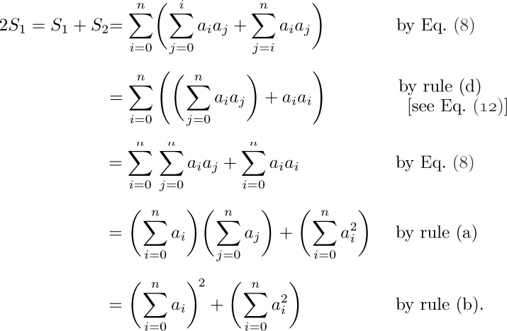
Four simple algebraic operations on sums are very important, and familiarity with them makes the solution of many problems possible. We shall now discuss these four operations.
a) The distributive law, for products of sums:

To understand this law, consider for example the special case

It is customary to drop the parentheses on the right-hand side of (4); a double summation such as  is written simply $∑_{R(i)}∑_{S(i)}a_{ij}$.
b) Change of variable:

This equation represents two kinds of transformations. In the first case we are simply changing the name of the index variable from i to j. The second case is more interesting: Here $p(j)$ is a function of j that represents a permutation of the relevant values; more precisely, for each integer i satisfying the relation $R(i)$, there must be exactly one integer j satisfying the relation $p(j)=i$. This condition is always satisfied in the important cases $p(j)=c+j$ and $p(j)=c-j$, where c is an integer not depending on j, and these are the cases used most frequently in applications. For example,

The reader should study this example carefully.
The replacement of j by $p(j)$ cannot be done for all infinite sums. The operation is always valid if $p(j)=c ± j$, as above, but in other cases some care must be used. [For example, see T. M. Apostol, Mathematical Analysis (Reading, Mass.: Addison–Wesley, 1957), Chapter 12. A sufficient condition to guarantee the validity of (5) for any permutation of the integers, $p(j)$, is that $∑_{R(j)}|a_{j}|$ exists.]
c) Interchanging order of summation:

Let us consider a very simple special case of this equation:

By Eq. (7), these two are equal; this says no more than

where we let $b_{i}=a_{i1}$ and $c_{i}=a_{i2}$.
The operation of interchanging the order of summation is extremely useful, since it often happens that we know a simple form for $∑_{R(i)}a_{ij}$, but not for $∑_{S(j)}a_{ij}$. We frequently need to interchange the summation order also in a more general situation, where the relation $S(j)$ depends on i as well as j. In such a case we can denote the relation by “$S(i,j)$.” The interchange of summation can always be carried out, in theory at least, as follows:

where $S'(j)$ is the relation “there is an integer i such that both $R(i)$ and $S(i,j)$ are true”; and $R'(i,j)$ is the relation “both $R(i)$ and $S(i,j)$ are true.” For example, if the summation is  , then $S'(j)$ is the relation “there is an integer i such that 1 ≤ i ≤ n and 1 ≤ j ≤ i,” that is, 1 ≤ j ≤ n; and $R'(i,j)$ is the relation “1 ≤ i ≤ n and 1 ≤ j ≤ i,” that is, j ≤ i ≤ n. Thus,

[Note: As in case (b), the operation of interchanging order of summation is not always valid for infinite series. If the series is absolutely convergent — that is, if $∑_{R(i)}∑_{S(j)}|a_{ij}|$ exists — it can be shown that Eqs. (7) and (9) are valid. Also if either one of $R(i)$ or $S(j)$ specifies a finite sum in Eq. (7), and if each infinite sum that appears is convergent, then the interchange is justified. In particular, Eq. (8) is always true for convergent infinite sums.]
d) Manipulating the domain. If $R(j)$ and $S(j)$ are arbitrary relations, we have

For example,

assuming that 1 ≤ m ≤ n. In this case “$R(j)$ and $S(j)$” is simply “j = m,” so we have reduced the second sum to simply “$a_{m}$.” In most applications of Eq. (11), either $R(j)$ and $S(j)$ are simultaneously satisfied for only one or two values of j, or else it is impossible to have both $R(j)$ and $S(j)$ true for the same j. In the latter case, the second sum on the right-hand side of Eq. (11) simply disappears.
Now that we have seen the four basic rules for manipulating sums, let’s study some further illustrations of how to apply these techniques.
Example 1.

The last step merely consists of simplifying the relations below the ∑’s.
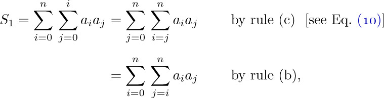
interchanging the names i and j and recognizing that $a_{j}a_{i}=a_{i}a_{j}$. If we denote the latter sum by $S_{2}$, we have
Thus we have derived the important identity

Example 3 (The sum of a geometric progression). Assume that x ≠ 1 and that n ≥ 0. Then
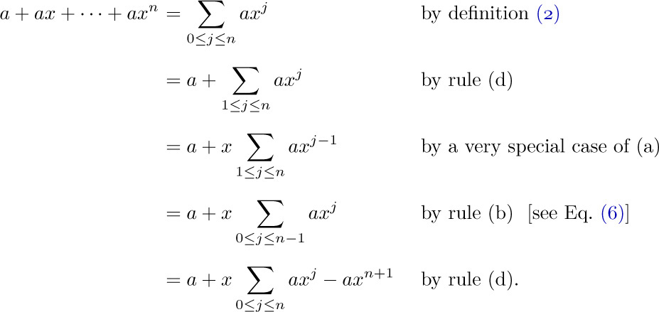
Comparing the first relation with the last, we have

hence we obtain the basic formula

Example 4 (The sum of an arithmetic progression). Assume that n ≥ 0. Then
since the first sum simply adds together $(n+1)$ terms that do not depend on j. Now by equating the first and last expressions and dividing by 2, we obtain

This is n + 1 times  , which can be understood as the number of terms times the average of the first and last terms.
Notice that we have derived the important equations (13), (14), and (15) purely by using simple manipulations of sums. Most textbooks would simply state those formulas, and prove them by induction. Induction is, of course, a perfectly valid procedure; but it does not give any insight into how on earth a person would ever have dreamed the formula up in the first place, except by some lucky guess. In the analysis of algorithms we are confronted with hundreds of sums that do not conform to any apparent pattern; by manipulating those sums, as above, we can often get the answer without the need for ingenious guesses.
Many manipulations of sums and other formulas become considerably simpler if we adopt the following bracket notation:

Then we can write, for example,

where the sum on the right is over all integers j, because the terms of that infinite sum are zero when $R(j)$ is false. (We assume that $a_{j}$ is defined for all j.)
With bracket notation we can derive rule (b) from rules (a) and (c) in an interesting way:

The remaining sum on j is equal to 1 when $R(i)$ is true, if we assume that p is a permutation of the relevant values as required in (5); hence we are left with  , which is
  . This proves (5). If p is not such a permutation, (18) tells us the true value of
  .
.
The most famous special case of bracket notation is the so-called Kronecker delta symbol,

introduced by Leopold Kronecker in 1868. More general notations such as (16) were introduced by K. E. Iverson in 1962; therefore (16) is often called Iverson’s convention. [See D. E. Knuth, AMM 99 (1992), 403–422.]
There is a notation for products, analogous to our notation for sums: The symbols

stand for the product of all $a_{j}$ for which the integer j satisfies $R(j)$. If no such integer j exists, the product is defined to have the value 1 (not 0).
Operations (b), (c), and (d) are valid for the ∏-notation as well as for the ∑-notation, with suitable simple modifications. The exercises at the end of this section give a number of examples of product notation in use.
We conclude this section by mentioning another notation for multiple summation that is often convenient: A single ∑-sign may be used with one or more relations in several index variables, meaning that the sum is taken over all combinations of variables that meet the conditions. For example,

This notation gives no preference to one index of summation over any other, so it allows us to derive (10) in a new way:

using the fact that $[1≤i≤n][1≤j≤i]=[1≤j≤i≤n]=[1≤j≤n][j≤i≤n]$. The more general equation (9) follows in a similar way from the identity

A further example that demonstrates the usefulness of summation with several indices is

where a is an n-tuply subscripted variable; for example, if n = 5 this notation stands for
$a_{11111}+a_{21110}+a_{22100}+a_{31100}+a_{32000}+a_{41000}+a_{50000}$.
(See the remarks on partitions of a number in Section 1.2.1.)
Exercises — First Set
![]() 1. [10] The text says that $a_{1}+a_{2}+···+a_{0}=0$. What, then, is $a_{2}+···+a_{0}$?
1. [10] The text says that $a_{1}+a_{2}+···+a_{0}=0$. What, then, is $a_{2}+···+a_{0}$?
2. [01] What does the notation $∑_{1≤j≤n}a_{j}$ mean, if $n=3.14$?
![]() 3. [13] Without using the ∑-notation, write out the equivalent of
3. [13] Without using the ∑-notation, write out the equivalent of

and also the equivalent of

Explain why the two results are different, in spite of rule (b).
4. [10] Without using the ∑-notation, write out the equivalent of each side of Eq. (10) as a sum of sums for the case n = 3.
![]() 5. [HM20] Prove that rule (a) is valid for arbitrary infinite series, provided that the series converge.
5. [HM20] Prove that rule (a) is valid for arbitrary infinite series, provided that the series converge.
6. [HM20] Prove that rule (d) is valid for an arbitrary infinite series, provided that any three of the four sums exist.
7. [HM23] Given that c is an integer, show that  even if both series are infinite.
8. [HM25] Find an example of infinite series in which Eq. (7) is false.
![]() 9. [05] Is the derivation of Eq. (14) valid even if n = −1?
9. [05] Is the derivation of Eq. (14) valid even if n = −1?
10. [05] Is the derivation of Eq. (14) valid even if n = −2?
11. [03] What should the right-hand side of Eq. (14) be if x = 1?
12. [10] What is 
13. [10] Using Eq. (15) and assuming that m ≤ n, evaluate  .
.
14. [11] Using the result of the previous exercise, evaluate  jk.
jk.
![]() 15. [M22] Compute the sum $1×2+2×2^{2}+3×2^{3}+···+n×2^{n}$ for small values of n. Do you see the pattern developing in these numbers? If not, discover it by manipulations similar to those leading up to Eq. (14).
15. [M22] Compute the sum $1×2+2×2^{2}+3×2^{3}+···+n×2^{n}$ for small values of n. Do you see the pattern developing in these numbers? If not, discover it by manipulations similar to those leading up to Eq. (14).
16. [M22] Prove that

if x ≠ 1, without using mathematical induction.
![]() 17. [M00] Let S be a set of integers. What is
17. [M00] Let S be a set of integers. What is 
18. [M20] Show how to interchange the order of summation as in Eq. (9) given that $R(i)$ is the relation “n is a multiple of i” and $S(i,j)$ is the relation “1 ≤ j < i.”
19. [20] What is 
![]() 20. [25] Dr. I. J. Matrix has observed a remarkable sequence of formulas: 9 × 1 + 2 = 11, 9 × 12 + 3 = 111, 9 × 123 + 4 = 1111, 9 × 1234 + 5 = 11111.
20. [25] Dr. I. J. Matrix has observed a remarkable sequence of formulas: 9 × 1 + 2 = 11, 9 × 12 + 3 = 111, 9 × 123 + 4 = 1111, 9 × 1234 + 5 = 11111.
a) Write the good doctor’s great discovery in terms of the ∑-notation.
b) Your answer to part (a) undoubtedly involves the number 10 as base of the decimal system; generalize this formula so that you get a formula that will perhaps work in any base b.
c) Prove your formula from part (b) by using formulas derived in the text or in exercise 16 above.
![]() 21. [M25] Derive rule (d) from (8) and (17).
21. [M25] Derive rule (d) from (8) and (17).
![]() 22. [20] State the appropriate analogs of Eqs. (5), (7), (8), and (11) for products instead of sums.
22. [20] State the appropriate analogs of Eqs. (5), (7), (8), and (11) for products instead of sums.
23. [10] Explain why it is a good idea to define $∑_{R(j)}a_{j}$ and $∏_{R(j)}a_{j}$ as zero and one, respectively, when no integers satisfy $R(j)$.
24. [20] Suppose that $R(j)$ is true for only finitely many j. By induction on the number of integers satisfying $R(j)$, prove that  , assuming that all $a_{j}\gt0$.
![]() 25. [15] Consider the following derivation; is anything amiss?
25. [15] Consider the following derivation; is anything amiss?

26. [25] Show that  may be expressed in terms of
  by manipulating the ∏-notation as stated in exercise 22.
27. [M20] Generalize the result of exercise 1.2.1–9 by proving that

assuming that $0 \lt a_{j}\lt 1$.
28. [M22] Find a simple formula for  .
.
![]() 29. [M30] (a) Express
29. [M30] (a) Express  in terms of the multiple-sum notation explained at the end of the section. (b) Express the same sum in terms of
  ,
,  , and
, and  [see Eq. (13)].
![]() 30. [M23] (J. Binet, 1812.) Without using induction, prove the identity
30. [M23] (J. Binet, 1812.) Without using induction, prove the identity

[An important special case arises when $w_{1},...,w_{n}$, $z_{1},...,z_{n}$ are arbitrary complex numbers and we set $a_{j}=w_{j}$,  ,
,  , $y_{j}=z_{j}$:

The terms  are nonnegative, so the famous Cauchy–Schwarz inequality

is a consequence of Binet’s formula.]
31. [M20] Use Binet’s formula to express the sum  in terms of
  ,
,  , and
, and  .
.
32. [M20] Prove that

![]() 33. [M30] One evening Dr. Matrix discovered some formulas that might even be classed as more remarkable than those of exercise 20:
33. [M30] One evening Dr. Matrix discovered some formulas that might even be classed as more remarkable than those of exercise 20:

Prove that these formulas are a special case of a general law; let $x_{1},x_{2},...,x_{n}$ be distinct numbers, and show that

34. [M25] Prove that
provided that 1 ≤ m ≤ n and x is arbitrary. For example, if n = 4 and m = 2, then

35. [HM20] The notation $\sup_{R(j)}a_{j}$ is used to denote the least upper bound of the elements $a_{j}$, in a manner exactly analogous to the ∑- and ∏-notations. (When $R(j)$ is satisfied for only finitely many j, the notation $\max_{R(j)}a_{j}$ is often used to denote the same quantity.) Show how rules (a), (b), (c), and (d) can be adapted for manipulation of this notation. In particular discuss the following analog of rule (a):

and give a suitable definition for the notation when $R(j)$ is satisfied for no j.
Exercises — Second Set
Determinants and matrices. The following interesting problems are for the reader who has experienced at least an introduction to determinants and elementary matrix theory. A determinant may be evaluated by astutely combining the operations of: (a) factoring a quantity out of a row or column; (b) adding a multiple of one row (or column) to another row (or column); (c) expanding by cofactors. The simplest and most often used version of operation (c) is to simply delete the entire first row and column, provided that the element in the upper left corner is +1 and the remaining elements in either the entire first row or the entire first column are zero; then evaluate the resulting smaller determinant. In general, the cofactor of an element $a_{ij}$ in an $n×n$ determinant is $(-1)^{i+j}$ times the $(n-1)×(n-1)$ determinant obtained by deleting the row and column in which $a_{ij}$ appeared. The value of a determinant is equal to $∑ a_{ij}·cofactor(a_{ij})$ summed with either i or j held constant and with the other subscript varying from 1 to n.
If $(b_{ij})$ is the inverse of matrix $(a_{ij})$, then $b_{ij}$ equals the cofactor of $a_{ji}$ (not $a_{ij}$), divided by the determinant of the whole matrix.
The following types of matrices are of special importance:

36. [M23] Show that the determinant of the combinatorial matrix is $x^{n−1}(x+ny)$.
![]() 37. [M24] Show that the determinant of Vandermonde’s matrix is
37. [M24] Show that the determinant of Vandermonde’s matrix is

![]() 38. [M25] Show that the determinant of Cauchy’s matrix is
38. [M25] Show that the determinant of Cauchy’s matrix is

39. [M23] Show that the inverse of a combinatorial matrix is a combinatorial matrix with the entries $b_{ij}=(-y+δ_{ij}(x+ny))/x(x+ny)$.
40. [M24] Show that the inverse of Vandermonde’s matrix is given by

Don’t be dismayed by the complicated sum in the numerator — it is just the coefficient of $x^{j-1}$ in the polynomial $(x_{1}-x)...(x_{n}-x)/(x_{i}-x)$.
41. [M26] Show that the inverse of Cauchy’s matrix is given by

42. [M18] What is the sum of all $n^{2}$ elements in the inverse of the combinatorial matrix?
43. [M24] What is the sum of all $n^{2}$ elements in the inverse of Vandermonde’s matrix? [Hint: Use exercise 33.]
![]() 44. [M26] What is the sum of all $n^{2}$ elements in the inverse of Cauchy’s matrix?
44. [M26] What is the sum of all $n^{2}$ elements in the inverse of Cauchy’s matrix?
![]() 45. [M25] A Hilbert matrix, sometimes called an $n×n$ segment of the (infinite) Hilbert matrix, is a matrix for which $a_{ij}=1/(i+j-1)$. Show that this is a special case of Cauchy’s matrix, find its inverse, show that each element of the inverse is an integer, and show that the sum of all elements of the inverse is $n^{2}$. [Note: Hilbert matrices have often been used to test various matrix manipulation algorithms, because they are numerically unstable, and they have known inverses. However, it is a mistake to compare the known inverse, given in this exercise, to the computed inverse of a Hilbert matrix, since the matrix to be inverted must be expressed in rounded numbers beforehand; the inverse of an approximate Hilbert matrix will be somewhat different from the inverse of an exact one, due to the instability present. Since the elements of the inverse are integers, and since the inverse matrix is just as unstable as the original, the inverse can be specified exactly, and one could try to invert the inverse. The integers that appear in the inverse are, however, quite large.] The solution to this problem requires an elementary knowledge of factorials and binomial coefficients, which are discussed in Sections 1.2.5 and 1.2.6.
45. [M25] A Hilbert matrix, sometimes called an $n×n$ segment of the (infinite) Hilbert matrix, is a matrix for which $a_{ij}=1/(i+j-1)$. Show that this is a special case of Cauchy’s matrix, find its inverse, show that each element of the inverse is an integer, and show that the sum of all elements of the inverse is $n^{2}$. [Note: Hilbert matrices have often been used to test various matrix manipulation algorithms, because they are numerically unstable, and they have known inverses. However, it is a mistake to compare the known inverse, given in this exercise, to the computed inverse of a Hilbert matrix, since the matrix to be inverted must be expressed in rounded numbers beforehand; the inverse of an approximate Hilbert matrix will be somewhat different from the inverse of an exact one, due to the instability present. Since the elements of the inverse are integers, and since the inverse matrix is just as unstable as the original, the inverse can be specified exactly, and one could try to invert the inverse. The integers that appear in the inverse are, however, quite large.] The solution to this problem requires an elementary knowledge of factorials and binomial coefficients, which are discussed in Sections 1.2.5 and 1.2.6.
![]() 46. [M30] Let A be an $m×n$ matrix, and let B be an $n×m$ matrix. Given that $1≤j_{1},j_{2},...,j_{m}≤n$, let $A_{j_{1}j_{2}...j_{m}}$ denote the $m×m$ matrix consisting of columns $j_{1},...,j_{m}$ of A, and let $B_{j_{1}j_{2}...j_{m}}$ denote the $m×m$ matrix consisting of rows $j_{1},...,j_{m}$ of B. Prove the Binet–Cauchy identity
46. [M30] Let A be an $m×n$ matrix, and let B be an $n×m$ matrix. Given that $1≤j_{1},j_{2},...,j_{m}≤n$, let $A_{j_{1}j_{2}...j_{m}}$ denote the $m×m$ matrix consisting of columns $j_{1},...,j_{m}$ of A, and let $B_{j_{1}j_{2}...j_{m}}$ denote the $m×m$ matrix consisting of rows $j_{1},...,j_{m}$ of B. Prove the Binet–Cauchy identity

(Note the special cases: (i) m = n, (ii) m = 1, (iii) $B=A^{T}$, (iv) m > n, (v) m = 2.)
47. [M27] (C. Krattenthaler.) Prove that

and generalize this equation to an identity for an $n×n$ determinant in $3n-2$ variables $x_{1},...,x_{n}$, $p_{1},...,p_{n−1}$, $q_{2},...,q_{n}$. Compare your formula to the result of exercise 38.
If x is any real number, we write
$\lfloor{x}\rfloor=$ the greatest integer less than or equal to x (the floor of x);
$\lceil{x}\rceil=$ the least integer greater than or equal to x (the ceiling of x).
The notation [x] was often used before 1970 for one or the other of these functions, usually the former; but the notations above, introduced by K. E. Iverson in the 1960s, are more useful, because $\lfloor{x}\rfloor$ and $\lceil{x}\rceil$ occur about equally often in practice. The function $\lfloor{x}\rfloor$ is sometimes called the entier function, from the French word for “integer.”.
The following formulas and examples are easily verified:

Exercises at the end of this section list other important formulas involving the floor and ceiling operations.
If x and y are any real numbers, we define the following binary operation:

From this definition we can see that, when y ≠ 0,

Consequently
a) if y > 0, then $0≤x\bmod y\lt y$;
b) if y < 0, then $0≥x\bmod y\gt y$;
c) the quantity $x-(x\bmod y)$ is an integral multiple of y.
We call $x\bmod y$ the remainder when x is divided by y; similarly, we call $\lfloor{x/y}\rfloor$ the quotient.
When x and y are integers, “mod” is therefore a familiar operation:

We have x mod y = 0 if and only if x is a multiple of y, that is, if and only if x is divisible by y. The notation $y{\setminus}x$, read “y divides x,” means that y is a positive integer and $x\bmod y=0$.
The “mod” operation is useful also when x and y take arbitrary real values. For example, with trigonometric functions we can write
$\tan x=\tan(x\bmod π)$.
The quantity $x\bmod 1$ is the fractional part of x; we have, by Eq. (1),

Writers on number theory often use the abbreviation “mod” in a different but closely related sense. We will use the following form to express the numbertheoretical concept of congruence: The statement

means that $x\bmod z=y\bmod z$; it is the same as saying that $x-y$ is an integral multiple of z. Expression (5) is read, “x is congruent to y modulo z.”
Let’s turn now to the basic elementary properties of congruences that will be used in the number-theoretical arguments of this book. All variables in the following formulas are assumed to be integers. Two integers x and y are said to be relatively prime if they have no common factor, that is, if their greatest common divisor is 1; in such a case we write $x⊥y$. The concept of relatively prime integers is a familiar one, since it is customary to say that a fraction is in “lowest terms” when the numerator is relatively prime to the denominator.
Law A. If $a≡b$ and $x≡y$, then $a ± x≡b ± y$ and $ax≡\md[by]{m}$.
Law B. If $ax≡by$ and $a≡b$, and if $a⊥m$, then $x≡\md[y]{m}$.
Law C. $a≡\md[b]{m}$ if and only if $an≡\md[bn]{mn}$, when n ≠ 0.
Law D. If $r⊥s$, then $a≡\md[b]{rs}$ if and only if $a≡\md[b]{r}$ and $a≡\md[b]{s}$.
Law A states that we can do addition, subtraction, and multiplication modulo m just as we do ordinary addition, subtraction, and multiplication. Law B considers the operation of division and shows that, when the divisor is relatively prime to the modulus, we can also divide out common factors. Laws C and D consider what happens when the modulus is changed. These laws are proved in the exercises below.
The following important theorem is a consequence of Laws A and B.
Theorem F (Fermat’s theorem, 1640). If p is a prime number, then $a^{p}≡\md[a]{p}$ for all integers a.
Proof. If a is a multiple of p, obviously $a^{p}≡0≡\md[a]{p}$. So we need only consider the case $a\bmod p≠0$. Since p is a prime number, this means that $a⊥p$. Consider the numbers

These p numbers are all distinct, for if $ax\bmod p=ay\bmod p$, then by definition (5) $ax≡\md[ay]{p}$; hence by Law B, $x≡\md[y]{p}$.
Since (6) gives p distinct numbers, all nonnegative and less than p, we see that the first number is zero and the rest are the integers $1,2,...,p-1$ in some order. Therefore by Law A,

Multiplying each side of this congruence by a, we obtain

and this proves the theorem, since each of the factors 1, 2, ..., p − 1 is relatively prime to p and can be canceled by Law B.
Exercises
1. [00] What are $\lfloor{1.1}\rfloor$, $\lfloor{−1.1}\rfloor$, $\lceil{−1.1}\rceil$, $\lfloor{0.99999}\rfloor$, and $\lfloor{\lg 35}\rfloor$?
![]() 2. [01] What is $\lceil{\lfloor{x}\rfloor}\rceil$?
2. [01] What is $\lceil{\lfloor{x}\rfloor}\rceil$?
3. [M10] Let n be an integer, and let x be a real number. Prove that
a) $\lfloor{x}\rfloor\lt n$ if and only if x < n;
b) $n≤\lfloor{x}\rfloor$ if and only if n ≤ x;
c) $\lceil{x}\rceil≤n$ if and only if x ≤ n;
d) $n\lt\lceil{x}\rceil$ if and only if n < x;
e) $\lfloor{x}\rfloor=n$ if and only if $x-1\lt n≤x$, and if and only if $n≤x\lt n+1$;
f) $\lceil{x}\rceil=n$ if and only if $x≤n\lt x+1$, and if and only if $n-1\lt x≤n$.
[These formulas are the most important tools for proving facts about $\lfloor{x}\rfloor$ and $\lceil{x}\rceil$.]
![]() 4. [M10] Using the previous exercise, prove that $\lfloor{−x}\rfloor=-\lceil{x}\rceil$.
4. [M10] Using the previous exercise, prove that $\lfloor{−x}\rfloor=-\lceil{x}\rceil$.
5. [16] Given that x is a positive real number, state a simple formula that expresses x rounded to the nearest integer. The desired rounding rule is to produce $\lfloor{x}\rfloor$ when $x\bmod  $, and to produce $\lceil{x}\rceil$ when $x\bmod
  $. Your answer should be a single formula that covers both cases. Discuss the rounding that would be obtained by your formula when x is negative.
![]() 6. [20] Which of the following equations are true for all positive real numbers x?
6. [20] Which of the following equations are true for all positive real numbers x?

7. [M15] Show that $\lfloor{x}\rfloor+\lfloor{y}\rfloor≤\lfloor{x+y}\rfloor$ and that equality holds if and only if $x\bmod 1 + y\bmod 1 \lt 1$. Does a similar formula hold for ceilings?
8. [00] What are $100\bmod 3$, $100\bmod 7$, $-100\bmod 7$, $-100\bmod 0$?
9. [05] What are $5\bmod -3$, $18\bmod -3$, $-2\bmod -3$?
![]() 10. [10] What are $1.1\bmod 1$, $0.11\bmod .1$, $0.11\bmod -.1$?
10. [10] What are $1.1\bmod 1$, $0.11\bmod .1$, $0.11\bmod -.1$?
11. [00] What does “$x≡\md[y]{0}$” mean by our conventions?
12. [00] What integers are relatively prime to 1?
13. [M00] By convention, we say that the greatest common divisor of 0 and n is $|n|$. What integers are relatively prime to 0?
![]() 14. [12] If $x\bmod 3=2$ and $x\bmod 5=3$, what is $x\bmod 15$?
14. [12] If $x\bmod 3=2$ and $x\bmod 5=3$, what is $x\bmod 15$?
15. [10] Prove that $z(x\bmod y)=(zx)\bmod (zy)$. [Law C is an immediate consequence of this distributive law.]
16. [M10] Assume that y > 0. Show that if $(x-z)/y$ is an integer and if 0 ≤ z < y, then $z=x\bmod y$.
17. [M15] Prove Law A directly from the definition of congruence, and also prove half of Law D: If $a≡\md[b]{rs}$, then $a≡\md[b]{r}$ and $a≡\md[b]{s}$. (Here r and s are arbitrary integers.)
18. [M15] Using Law B, prove the other half of Law D: If $a≡\md[b]{r}$ and $a≡\md[b]{s}$, then $a≡\md[b]{rs}$, provided that $r⊥s$.
![]() 19. [M10] (Law of inverses.) If $n⊥m$, there is an integer n′ such that $nn'≡\md[ 1]{m}$. Prove this, using the extension of Euclid’s algorithm (Algorithm 1.2.1E).
19. [M10] (Law of inverses.) If $n⊥m$, there is an integer n′ such that $nn'≡\md[ 1]{m}$. Prove this, using the extension of Euclid’s algorithm (Algorithm 1.2.1E).
20. [M15] Use the law of inverses and Law A to prove Law B.
21. [M22] (Fundamental theorem of arithmetic.) Use Law B and exercise 1.2.1–5 to prove that every integer n > 1 has a unique representation as a product of primes (except for the order of the factors). In other words, show that there is exactly one way to write $n=p_{1}p_{2}...p_{k}$, where each $p_{j}$ is prime and $p_{1}≤p_{2}≤···≤p_{k}$.
![]() 22. [M10] Give an example to show that Law B is not always true if a is not relatively prime to m.
22. [M10] Give an example to show that Law B is not always true if a is not relatively prime to m.
23. [M10] Give an example to show that Law D is not always true if r is not relatively prime to s.
![]() 24. [M20] To what extent can Laws A, B, C, and D be generalized to apply to arbitrary real numbers instead of integers?
24. [M20] To what extent can Laws A, B, C, and D be generalized to apply to arbitrary real numbers instead of integers?
25. [M02] Show that, according to Theorem F, $a^{p-1}\bmod p=$ [a is not a multiple of p], whenever p is a prime number.
26. [M15] Let p be an odd prime number, let a be any integer, and let $b=a^{(p-1)/2}$. Show that $b\bmod p$ is either 0 or 1 or $p-1$. [Hint: Consider $(b+1)(b-1)$.]
27. [M15] Given that n is a positive integer, let $φ(n)$ be the number of values among $\{0,1,...,n-1\}$ that are relatively prime to n. Thus $φ(1)=1$, $φ(2)=1$, $φ(3)=2$, $φ(4)=2$, etc. Show that $φ(p)=p-1$ if p is a prime number; and evaluate $φ(p^{e})$, when e is a positive integer.
![]() 28. [M25] Show that the method used to prove Theorem F can be used to prove the following extension, called Euler’s theorem: $a^{φ(m)}≡\md[1]{m}$, for any positive integer m, when $a⊥m$. (In particular, the number n′ in exercise 19 may be taken to be $n^{φ(m)-1}\bmod m$.)
28. [M25] Show that the method used to prove Theorem F can be used to prove the following extension, called Euler’s theorem: $a^{φ(m)}≡\md[1]{m}$, for any positive integer m, when $a⊥m$. (In particular, the number n′ in exercise 19 may be taken to be $n^{φ(m)-1}\bmod m$.)
29. [M22] A function $f(n)$ of positive integers n is called multiplicative if $f(rs)=f(r)f(s)$ whenever $r⊥s$. Show that each of the following functions is multiplicative: (a) $f(n)=n^{c}$, where c is any constant; (b) $f(n)=$ [n is not divisible by $k^{2}$ for any integer k > 1]; (c) $f(n)=c^{k}$, where k is the number of distinct primes that divide n; (d) the product of any two multiplicative functions.
30. [M30] Prove that the function $φ(n)$ of exercise 27 is multiplicative. Using this fact, evaluate φ(1000000), and give a method for evaluating $φ(n)$ in a simple way once n has been factored into primes.
31. [M22] Prove that if f (n) is multiplicative, so is $g(n)=∑_{d\setminus n}f(d)$.
32. [M18] Prove the double-summation identity

for any function $f(x,y)$.
33. [M18] Given that m and n are integers, evaluate (a)  ; (b)
; (b)  . (The special case m = 0 is worth noting.)
![]() 34. [M21] What conditions on the real number b > 1 are necessary and sufficient to guarantee that $\lfloor{log_{b}x}\rfloor=\lfloor{log_{b}\lfloor{x}\rfloor}\rfloor$ for all real x ≥ 1?
34. [M21] What conditions on the real number b > 1 are necessary and sufficient to guarantee that $\lfloor{log_{b}x}\rfloor=\lfloor{log_{b}\lfloor{x}\rfloor}\rfloor$ for all real x ≥ 1?
![]() 35. [M20] Given that m and n are integers and n > 0, prove that
35. [M20] Given that m and n are integers and n > 0, prove that
$\lfloor{(x+m)/n}\rfloor=\lfloor{(\lfloor{x}\rfloor+m)/n}\rfloor$
for all real x. (When m = 0, we have an important special case.) Does an analogous result hold for the ceiling function?
36. [M23] Prove that  ; also evaluate
  .
.
![]() 37. [M30] Let m and n be integers, n > 0. Show that
37. [M30] Let m and n be integers, n > 0. Show that

where d is the greatest common divisor of m and n, and x is any real number.
38. [M26] (E. Busche, 1909.) Prove that, for all real x and y with y > 0,

In particular, when y is a positive integer n, we have the important formula

39. [HM35] A function f for which  , whenever n is a positive integer, is called a replicative function. The previous exercise establishes the fact that $\lfloor{x}\rfloor$ is replicative. Show that the following functions are replicative:
a)  ;
;
b) $f(x)=$ [x is an integer];
c) $f(x)=$ [x is a positive integer];
d) $f(x)=$ [there exists a rational number r and an integer m such that $x=rπ+m$];
e) three other functions like the one in (d), with r and/or m restricted to positive values;
f) $f(x)=\log|2\sin πx|$, if the value $f(x)=-∞$ is allowed;
g) the sum of any two replicative functions;
h) a constant multiple of a replicative function;
i) the function $g(x)=f(x-\lfloor{x}\rfloor)$, where $f(x)$ is replicative.
40. [HM46] Study the class of replicative functions; determine all replicative functions of a special type. For example, is the function in (a) of exercise 39 the only continuous replicative function? It may be interesting to study also the more general class of functions for which

Here $a_{n}$ and $b_{n}$ are numbers that depend on n but not on x. Derivatives and (if $b_{n}=0$) integrals of these functions are of the same type. If we require that $b_{n}=0$, we have, for example, the Bernoulli polynomials, the trigonometric functions $\cot πx$ and $\csc^{2}πx$, as well as Hurwitz’s generalized zeta function  for fixed s. With $b_{n}≠0$ we have still other well-known functions, such as the psi function.
41. [M23] Let $a_{1},a_{2},a_{3},...$ be the sequence 1, 2, 2, 3, 3, 3, 4, 4, 4, 4, ...; find an expression for $a_{n}$ in terms of n, using the floor and/or ceiling function.
42. [M24] (a) Prove that

(b) The preceding formula is useful for evaluating certain sums involving the floor function. Prove that, if b is an integer ≥ 2,

43. [M23] Evaluate  .
.
44. [M24] Show that  , if b and n are integers, n ≥ 0, and b ≥ 2. What is the value of this sum when n < 0?
![]() 45. [M28] The result of exercise 37 is somewhat surprising, since it implies that
45. [M28] The result of exercise 37 is somewhat surprising, since it implies that

when m and n are positive integers and x is arbitrary. This “reciprocity relationship” is one of many similar formulas (see Section 3.3.3). Show that in general we have

for any function f and all integers m, n > 0. In particular, prove that

[Hint: Consider the change of variable $r=\lfloor{mj/n}\rfloor$. Binomial coefficients  are discussed in Section 1.2.6.]
46. [M29] (General reciprocity law.) Extend the formula of exercise 45 to obtain an expression for  , where α is any positive real number.
![]() 47. [M31] When p is an odd prime number, the Legendre symbol
47. [M31] When p is an odd prime number, the Legendre symbol  is defined to be +1, 0, or −1, depending on whether $q^{(p-1)/2}\bmod p$ is 1, 0, or p − 1. (Exercise 26 proves that these are the only possible values.)
a) Given that q is not a multiple of p, show that the numbers
$(-1)^{\lfloor{2kq/p}\rfloor}(2kq\bmod p)$, $0\lt k\lt p/2$,
are congruent in some order to the numbers $2,4,...,p-\md[1]{p}$. Hence  where
where  .
.
b) Use the result of (a) to calculate  .
.
c) Given that q is odd, show that  unless q is a multiple of p. [Hint: Consider the quantity $\lfloor{(p-1-2k)q/p}\rfloor$.]
d) Use the general reciprocity formula of exercise 46 to obtain the law of quadratic reciprocity,  , given that p and q are distinct odd primes.
48. [M26] Prove or disprove the following identities, for integers m and n:

49. [M30] Suppose the integer-valued function $f(x)$ satisfies the two simple laws (i) $f(x+1)=f(x)+1$; (ii) $f(x)=f(f(nx)/n)$ for all positive integers n. Prove that either $f(x)=\lfloor{x}\rfloor$ for all rational x, or $f(x)=\lceil{x}\rceil$ for all rational x.
A permutation of n objects is an arrangement of n distinct objects in a row. There are six permutations of three objects $\{a,b,c\}$:

The properties of permutations are of great importance in the analysis of algorithms, and we will deduce many interesting facts about them later in this book.* Our first task is simply to count them: How many permutations of n objects are possible? There are n ways to choose the leftmost object, and once this choice has been made there are $n-1$ ways to select a different object to place next to it; this gives us $n(n-1)$ choices for the first two positions. Similarly, we find that there are $n-2$ choices for the third object distinct from the first two, and a total of $n(n-1)(n-2)$ possible ways to choose the first three objects. In general, if $p_{nk}$ denotes the number of ways to choose k objects out of n and to arrange them in a row, we see that

The total number of permutations is therefore $p_{nn}=n(n-1)...(1)$.
* In fact, permutations are so important, Vaughan Pratt has suggested calling them “perms.” As soon as Pratt’s convention is established, textbooks of computer science will be somewhat shorter (and perhaps less expensive).
The process of constructing all permutations of n objects in an inductive manner, assuming that all permutations of n − 1 objects have been constructed, is very important in our applications. Let us rewrite (1) using the numbers $\{1,2,3\}$ instead of the letters $\{a,b,c\}$; the permutations are then

Consider how to get from this array to the permutations of $\{1,2,3,4\}$. There are two principal ways to go from n − 1 objects to n objects.
Method 1. For each permutation $a_{1}a_{2}...a_{n-1}$ of $\{1,2,...,n-1\}$, form n others by inserting the number n in all possible places, obtaining
$n a_{1}a_{2}...a_{n-1}$, $a_{1}n a_{2}...a+{n-1}$, $...,$ $a_{1}a_{2}...n a_{n-1}$, $a_{1}a_{2}...a_{n-1}n$.
For example, from the permutation 2 3 1 in (3), we get 4 2 3 1, 2 4 3 1, 2 3 4 1, 2 3 1 4. It is clear that all permutations of n objects are obtained in this manner and that no permutation is obtained more than once.
Method 2. For each permutation $a_{1}a_{2}...a_{n-1}$ of $\{1,2,...,n-1\}$, form n others as follows: First construct the array

Then rename the elements of each permutation using the numbers $\{1,2,...,n\}$, preserving order. For example, from the permutation 2 3 1 in (3) we get

and, renaming, we get
3 4 2 1, 3 4 1 2, 2 4 1 3, 2 3 1 4.
Another way to describe this process is to take the permutation $a_{1}a_{2}...a_{n-1}$ and a number k, 1 ≤ k ≤ n; add one to each $a_{j}$ whose value is ≥ k, thus obtaining a permutation $b_{1}b_{2}...b_{n-1}$ of the elements $\{1,...,k-1,k+1,...,n\}$; then $b_{1}b_{2}...b_{n-1}k$ is a permutation of $\{1,...,n\}$.
Again it is clear that we obtain each permutation of n elements exactly once by this construction. Putting k at the left instead of the right, or putting k in any other fixed position, would obviously work just as well.
If $p_{n}$ is the number of permutations of n objects, both of these methods show that $p_{n}=np_{n-1}$; this offers us two further proofs that $p_{n}=n(n-1)...(1)$, as we already established in Eq. (2).
The important quantity $p_{n}$ is called n factorial and it is written

Our convention for vacuous products (Section 1.2.3) gives us the value

and with this convention the basic identity

is valid for all positive integers n.
Factorials come up sufficiently often in computer work that the reader is advised to memorize the values of the first few:
$0!=1$, $1!=1$, $2!=2$, $3!=6$, $4!=24$, $5!=120$.
The factorials increase very rapidly; for example, $1000!$ is an integer with over 2500 decimal digits.
It is helpful to keep the value $10!=3,628,800$ in mind; one should remember that 10! is about  . In a sense, this number represents an approximate dividing line between things that are practical to compute and things that are not. If an algorithm requires the testing of more than 10! cases, it may consume too much computer time to be practical. On the other hand, if we decide to test $10!$ cases and each case requires, say, one millisecond of computer time, then the entire run will take about an hour. These comments are very vague, of course, but they can be useful to give an intuitive idea of what is computationally feasible.
It is only natural to wonder what relation n! bears to other quantities in mathematics. Is there any way to tell how large 1000! is, without laboriously carrying out the multiplications implied in Eq. (4)? The answer was found by James Stirling in his famous work Methodus Differentialis (1730), page 137; we have

The “≈” sign that appears here denotes “approximately equal,” and “e” is the base of natural logarithms introduced in Section 1.2.2. We will prove Stirling’s approximation (7) in Section 1.2.11.2. Exercise 24 gives a simple proof of a less precise result.
As an example of the use of this formula, we may compute

In this case the error is about 1%; we will see later that the relative error is approximately $1/(12n)$.
In addition to the approximate value given by Eq. (7), we can also rather easily obtain the exact value of n! factored into primes. In fact, the prime p is a divisor of $n!$ with the multiplicity

For example, if n = 1000 and p = 3, we have

so $1000!$ is divisible by $3^{498}$ but not by $3^{499}$. Although formula (8) is written as an infinite sum, it is really finite for any particular values of n and p, because all of the terms are eventually zero. It follows from exercise 1.2.4–35 that $\lfloor{n/p^{k+1}}\rfloor=\lfloor{\lfloor{n/p^{k}}\rfloor/p}\rfloor$; this fact facilitates the calculation in Eq. (8), since we can just divide the value of the previous term by p and discard the remainder.
Equation (8) follows from the fact that $\lfloor{n/p^{k}}\rfloor$ is the number of integers among $\{1,2,...,n\}$ that are multiples of $p^{k}$. If we study the integers in the product (4), any integer that is divisible by $p^{j}$ but not by $p^{j+1}$ is counted exactly j times: once in $\lfloor{n/p}\rfloor$, once in $\lfloor{n/p^{2}}\rfloor,...,$ once in $\lfloor{n/p^{j}}\rfloor$. This accounts for all occurrences of p as a factor of $n!$. [See A. M. Legendre, Essai sur la Théorie des Nombres, second edition (Paris: 1808), page 8.]
Another natural question arises: Now that we have defined n! for non-negative integers n, perhaps the factorial function is meaningful also for rational values of n, and even for real values. What is  , for example? Let us illustrate this point by introducing the “termial” function

which is analogous to the factorial function except that we are adding instead of multiplying. We already know the sum of this arithmetic progression from Eq. 1.2.3–(15):

This suggests a good way to generalize the “termial” function to arbitrary n, by using (10) instead of (9). We have  .
.
Stirling himself made several attempts to generalize n! to noninteger n. He extended the approximation (7) into an infinite sum, but unfortunately the sum did not converge for any value of n; his method gave extremely good approximations, but it couldn’t be extended to give an exact value. [For a discussion of this somewhat unusual situation, see K. Knopp, Theory and Application of Infinite Series, 2nd ed. (Glasgow: Blackie, 1951), 518–520, 527, 534.]
Stirling tried again, by noticing that

(We will prove this formula in the next section.) The apparently infinite sum in Eq. (11) is in reality finite for any nonnegative integer n; however, it does not provide the desired generalization of n!, since the infinite sum does not exist except when n is a nonnegative integer. (See exercise 16.)
Still undaunted, Stirling found a sequence $a_{1},a_{2},...$ such that

He was unable to prove that this sum defined n! for all fractional values of n, although he was able to deduce the value of  .
.
At about the same time, Leonhard Euler considered the same problem, and he was the first to find the appropriate generalization:

Euler communicated this idea in a letter to Christian Goldbach on October 13, 1729. His formula defines n! for any value of n except negative integers (when the denominator becomes zero); in such cases n! is taken to be infinite. Exercises 8 and 22 explain why Eq. (13) is a reasonable definition.
Nearly two centuries later, in 1900, C. Hermite proved that Stirling’s idea (12) actually does define n! successfully for nonintegers n, and that in fact Euler’s and Stirling’s generalizations are identical.
Many notations were used for factorials in the early days. Euler actually wrote [n], Gauss wrote Π n, and the symbols  and
and  were popular in England and Italy. The notation n!, which is universally used today when n is an integer, was introduced by a comparatively little known mathematician, Christian Kramp, in an algebra text [Élémens d’Arithmétique Universelle (Cologne: 1808), page 219].
When n is not an integer, however, the notation n! is less common; instead we customarily employ a notation due to A. M. Legendre:

This function $Γ(x)$ is called the gamma function, and by Eq. (13) we have the definition

A graph of $Γ(x)$ is shown in Fig. 7.

Fig. 7. The function Γ (x) = (x - 1)!. The local minimum at X has the coordinates (1.46163 21449 68362 34126 26595, 0.88560 31944 10888 70027 88159).
Equations (13) and (15) define factorials and the gamma function for complex values as well as real values; but we generally use the letter z, instead of n or x, when thinking of a variable that has both real and imaginary parts. The factorial and gamma functions are related not only by the rule $z!=Γ(z+1)$ but also by

which holds whenever z is not an integer. (See exercise 23.)
Although $Γ(z)$ is infinite when z is zero or a negative integer, the function $1/Γ(z)$ is well defined for all complex z. (See exercise 1.2.7–2.) Advanced applications of the gamma function often make use of an important contour integral formula due to Hermann Hankel:

the path of complex integration starts at −∞, then circles the origin in a counterclockwise direction and returns to −∞. [Zeitschrift für Math. und Physik 9 (1864), 1–21.]
Many formulas of discrete mathematics involve factorial-like products known as factorial powers. The quantities  and
and  (read, “x to the k falling” and “x to the k rising”) are defined as follows, when k is a positive integer:


Thus, for example, the number $p_{nk}$ of (2) is just  . Notice that we have

The general formulas

can be used to define factorial powers for other values of k. [The notations and are due respectively to A. Capelli, Giornale di Mat. di Battaglini 31 (1893), 291–313, and L. Toscano, Comment. Accademia della Scienze 3 (1939), 721–757.]
The interesting history of factorials from the time of Stirling to the present day is traced in an article by P. J. Davis, “Leonhard Euler’s integral: A historical profile of the gamma function,” AMM 66 (1959), 849–869. See also J. Dutka, Archive for History of Exact Sciences 31 (1984), 15–34.