2. [10] In the notation of Eq. (2), show that $p_{n(n-1)}=p_{nn}$, and explain why this happens.

3. [10] What permutations of ${1, 2, 3, 4, 5}$ would be constructed from the permutation 3 1 2 4 using Methods 1 and 2, respectively?

4. [13] Given the fact that log₁₀ 1000! = 2567.60464 ..., determine exactly how many decimal digits are present in the number 1000!. What is the most significant digit? What is the least significant digit?

5. [15] Estimate 8! using the following more exact version of Stirling’s approximation:

7. [M10] Show that the “generalized termial” function in Eq. (10) satisfies the identity $x?=x+(x-1)$? for all real numbers x.

8. [HM15] Show that the limit in Eq. (13) does equal $n!$ when n is a nonnegative integer.

10. [HM20] Does the identity $Γ (x+1)=xΓ (x)$ hold for all real numbers x? (See exercise 7.)

11. [M15] Let the representation of n in the binary system be $n=2^{e_{1}}+2^{e_{2}}+...+2^{e_{r}}$ where $e_{1}\gt e_{2}\gt...\gt e_{r} ≥ 0$. Show that $n!$ is divisible by $2^{n-r}$ but not by $2^{n-r+1}$.

12. [M22] (A. Legendre, 1808.) Generalizing the result of the previous exercise, let p be a prime number, and let the representation of n in the p-ary number system be $n=a_{k}p^{k}+a_{k-1}p^{k-1}+...+a_{1}p+a_{0}$. Express the number μ of Eq. (8) in a simple formula involving n, p, and a’s.

13. [M23] (Wilson’s theorem, actually due to Leibniz, 1682.) If p is prime, then $(p-1)!\bmod p=p-1$. Prove this, by pairing off numbers among ${1, 2,..., p-1}$ whose product modulo p is 1.

14. [M28] (L. Stickelberger, 1890.) In the notation of exercise 12, we can determine $n!\bmod p$ in terms of the p-ary representation, for any positive integer n, thus generalizing Wilson’s theorem. In fact, prove that $n!/p^{μ}≡(-1)^{μ}a_{0} ! a_{1} !... a_{k} ! (modulo p)$.

15. [HM15] The permanent of a square matrix is defined by the same expansion as the determinant except that each term of the permanent is given a plus sign while the determinant alternates between plus and minus. Thus the permanent of

16. [HM15] Show that the infinite sum in Eq. (11) does not converge unless n is a nonnegative integer.

equals $Γ (1+β_{1})... Γ (1+β_{k}) /Γ (1+α_{1})... Γ (1+α_{k}), if α_{1}+···+α_{k}=β_{1}+···+β_{k}$ and if none of the β’s is a negative integer.

18. [M20] Assume that

. (This is “Wallis’s product,” obtained by J. Wallis in 1655, and we will prove it in exercise 1.2.6–43.) Using the previous exercise, prove that

19. [HM22] Denote the quantity appearing after “$\lim_{m→∞}$” in Eq. (15) by $Γ_{m}(x)$. Show that

20. [HM21] Using the fact that $0≤e^{-t}-(1-t/m)^{m}≤t^{2}e^{-t}/m$, if 0 ≤ t ≤ m, and the previous exercise, show that

, if x > 0.

21. [HM25] (L. F. A. Arbogast, 1800.) Let

represent the kth derivative of a function u with respect to x. The chain rule states that

. If we apply this to second derivatives, we find

. Show that the general formula is

22. [HM20] Try to put yourself in Euler’s place, looking for a way to generalize n! to noninteger values of n. Since

times

equals $(n+1)!/n!=n+1$, it seems natural that

should be approximately

. Similarly,

should be

. Invent a hypothesis about the ratio $(n+x)!/n!$ as n approaches infinity. Is your hypothesis correct when x is an integer? Does it tell anything about the appropriate value of $x!$ when x is not an integer?

25. [M20] Do factorial powers satisfy a law analogous to the ordinary law of exponents, $x^{m+n}=x^{m}x^{n}$?

1.2.6. Binomial Coefficients

The combinations of n objects taken k at a time are the possible choices of k different elements from a collection of n objects, disregarding order. The combinations of the five objects ${a, b, c, d, e}$ taken three at a time are

It is a simple matter to count the total number of k-combinations of n objects: Equation (2) of the previous section told us that there are $n(n-1)... (n-k+1)$ ways to choose the first k objects for a permutation; and every k-combination appears exactly $k!$ times in these arrangements, since each combination appears in all its permutations. Therefore the number of combinations, which we denote by

, is

The quantity

, read “n choose k,” is called a binomial coefficient; these numbers have an extraordinary number of applications. They are probably the most important quantities entering into the analysis of algorithms, so the reader is urged to become familiar with them.

Equation (2) may be used to define

even when n is not an integer. To be precise, we define the symbol

for all real numbers r and all integers k as follows:

Table 1 gives values of the binomial coefficients for small integer values of r and k; the values for 0 ≤ r ≤ 4 should be memorized.

Table 1 Table of Binomial Coefficients (Pascal’s Triangle)

Binomial coefficients have a long and interesting history. Table 1 is called “Pascal’s triangle” because it appeared in Blaise Pascal’s Traité du Triangle Arithmétique in 1653. This treatise was significant because it was one of the first works on probability theory, but Pascal did not invent the binomial coefficients (which were well-known in Europe at that time). Table 1 also appeared in the treatise Szu-yüan Yü-chien (“The Precious Mirror of the Four Elements”) by the Chinese mathematician Chu Shih-Chieh in 1303, where they were said to be an old invention. Yang Hui, in 1261, credited them to Chia Hsien (c. 1100), whose work is now lost. The earliest known detailed discussion of binomial coefficients is in a tenth-century commentary, due to Halāyudha, on an ancient Hindu classic, Pi

gala’s Chandaśāstra. [See G. Chakravarti, Bull. Calcutta Math. Soc. 24 (1932), 79–88.] Another Indian mathematician, Mahāvīra, had previously explained rule (3) for computing

in Chapter 6 of his Gan. ita Sāra Sagraha, written about 850; and in 1150 Bhāskara repeated Mahāvīra’s rule near the end of his famous book Līlāvatī. For small values of k, binomial coefficients were known much earlier; they appeared in Greek and Roman writings with a geometric interpretation (see Fig. 8). The notation

was introduced by Andreas von Ettingshausen in §31 of his book Die combinatorische Analysis (Vienna: 1826).

The reader has probably noticed several interesting patterns in Table 1. Binomial coefficients satisfy literally thousands of identities, and for centuries their amazing properties have been continually explored. In fact, there are so many relations present that when someone finds a new identity, not many people get excited about it any more, except the discoverer. In order to manipulate the formulas that arise in the analysis of algorithms, a facility for handling binomial coefficients is a must, and so an attempt has been made in this section to explain in a simple way how to maneuver with these numbers. Mark Twain once tried to reduce all jokes to a dozen or so primitive kinds (farmer’s daughter, mother-in-law, etc.); we will try to condense the thousands of identities into a small set of basic operations with which we can solve nearly every problem involving binomial coefficients that we will meet.

In most applications, both of the numbers r and k that appear in

will be integers, and some of the techniques we will describe are applicable only in such cases. Therefore we will be careful to list, at the right of each numbered equation, any restrictions on the variables that appear. For example, Eq. (3) mentions the requirement that k is an integer; there is no restriction on r. The identities with fewest restrictions are the most useful.

This allows combinations of factorials to be represented as binomial coefficients and conversely.

This formula holds for all integers k. When k is negative or greater than n, the binomial coefficient is zero (provided that n is a nonnegative integer).

This formula is very useful for combining a binomial coefficient with other parts of an expression. By elementary transformation we have the rules

the first of which is valid for all integers k, and the second when no division by zero has been performed. We also have a similar relation:

Let us illustrate these transformations, by proving Eq. (8) using Eqs. (6) and (7) alternately:

[Note: This derivation is valid only when r is a positive integer ≠ k, because of the constraints involved in Eqs. (6) and (7); yet Eq. (8) claims to be valid for arbitrary r ≠ k. This can be proved in a simple and important manner: We have verified that

for infinitely many values of r. Both sides of this equation are polynomials in r. A nonzero polynomial of degree n can have at most n distinct zeros; so (by subtraction) if two polynomials of degree ≤ n agree at n + 1 or more different points, the polynomials are identically equal. This principle may be used to extend the validity of many identities from integers to all real numbers.]

is clearly valid in Table 1 (every value is the sum of the two values above and to the left) and we may easily verify it in general from Eq. (3). Alternatively, Eqs. (7) and (8) tell us that

Equation (9) is often useful in obtaining proofs by induction on r, when r is an integer.

Thus we are led to two important summation formulas that can be expressed as follows:

Equation (11) can easily be proved by induction on n, but it is interesting to see how it can also be derived from Eq. (10) with two applications of Eq. (6):

Equation (11) occurs very frequently in applications; in fact, we have already derived special cases of it in previous sections. For example, when m = 1, we have our old friend, the sum of an arithmetic progression:

Suppose that we want a simple formula for the sum $1^{2}+2^{2}+···+n^{2}$. This can be obtained by observing that

; hence

And this answer, obtained in terms of binomial coefficients, can be put back into polynomial notation if desired:

The sum $1^{3}+2^{3}+···+n^{3}$ can be obtained in a similar way; any polynomial $a_{0}+a_{1}k+a_{2}k^{2}+···+a_{m}k^{m}$ can be expressed as

for suitably chosen coefficients $b_{0},..., b_{m}$. We will return to this subject later.

F. The binomial theorem. Of course, the binomial theorem is one of our principal tools:

For example, $(x+y)^{4}=x^{4}+4x^{3}y+6x^{2}y^{2}+4xy^{3}+y^{4}$. (At last we are able to justify the name “binomial coefficient” for the numbers

It is important to notice that we have written ∑_k in Eq. (13), rather than

as might have been expected. If no restriction is placed on k, we are summing over all integers, $-∞\lt k\lt +∞$; but the two notations are exactly equivalent in this case, since the terms in Eq. (13) are zero when k < 0 or k > r. The simpler form $∑_{k}$ is to be preferred, since all manipulations with sums are simpler when the conditions of summation are simpler. We save a good deal of tedious effort if we do not need to keep track of the lower and/or upper limits of summation, so the limits should be left unspecified whenever possible. Our notation has another advantage also: If r is not a nonnegative integer, Eq. (13) becomes an infinite sum, and the binomial theorem of calculus states that Eq. (13) is valid for all r, if |x/y| < 1.

The discovery of the binomial theorem was announced by Isaac Newton in letters to Oldenburg on June 13, 1676 and October 24, 1676. [See D. Struik, Source Book in Mathematics (Harvard Univ. Press, 1969), 284–291.] But he apparently had no real proof of the formula; at that time the necessity for rigorous proof was not fully realized. The first attempted proof was given by L. Euler in 1774, although his effort was incomplete. Finally, C. F. Gauss gave the first actual proof in 1812. In fact, Gauss’s work represented the first time anything about infinite sums was proved satisfactorily.

Early in the nineteenth century, N. H. Abel found a surprising generalization of the binomial formula (13):

This is an identity in three variables, x, y, and z (see exercises 50 through 52). Abel published and proved this formula in Volume 1 of A. L. Crelle’s soon-to-be-famous Journal für die reine und angewandte Mathematik (1826), pages 159–160. It is interesting to note that Abel contributed many other papers to the same Volume 1, including his famous memoirs on the unsolvability of algebraic equations of degree 5 or more by radicals, and on the binomial theorem. See H. W. Gould, AMM 69 (1962), 572, for a number of references to Eq. (16).

follows immediately from the definition (3) when each term of the numerator is negated. This is often a useful transformation on the upper index.

This identity could be proved by induction using Eq. (9), but we can use Eqs. (17) and (10) directly:

(Set r = n and k = n − m in Eq. (17) and use (6).) We have moved n from the upper position to the lower.

H. Simplifying products. When products of binomial coefficients appear, they can usually be reexpressed in several different ways by expanding into factorials and out again using Eq. (5). For example,

It suffices to prove Eq. (20) when r is an integer ≥ m (see the remarks after Eq. (8)), and when 0 ≤ k ≤ m. Then

Equation (20) is very useful when an index (namely m) appears in both the upper and the lower position, and we wish to have it appear in one place rather than two. Notice that Eq. (7) is the special case of Eq. (20) when k = 1.

I. Sums of products. To complete our set of binomial-coefficient manipulations, we present the following very general identities, which are proved in the exercises at the end of this section. These formulas show how to sum over a product of two binomial coefficients, considering various places where the running variable k might appear:

Of these identities, Eq. (21) is by far the most important, and it should be memorized. One way to remember it is to interpret the right-hand side as the number of ways to select n people from among r men and s women; each term on the left is the number of ways to choose k of the men and n − k of the women. Equation (21) is commonly called Vandermonde’s convolution, since A. Vandermonde published it in Mém. Acad. Roy. Sciences (Paris, 1772), part 1, 489–498. However, it had appeared already in Chu Shih-Chieh’s 1303 treatise mentioned earlier [see J. Needham, Science and Civilisation in China 3 (Cambridge University Press, 1959), 138–139].

If $r=tk$ in Eq. (26), we avoid the zero denominator by canceling with a factor in the numerator; therefore Eq. (26) is a polynomial identity in the variables r, s, t. Obviously Eq. (21) is a special case of Eq. (26) with t = 0.

We should point out a nonobvious use of Eqs. (23) and (25): It is often helpful to replace the simple binomial coefficient on the right-hand side by the more complicated expression on the left, interchange the order of summation, and simplify. We may regard the left-hand sides as expansions of

This completes our study of binomial-coefficientology. The reader is advised to learn especially Eqs. (5), (6), (7), (9), (13), (17), (20), and (21) — frame them with your favorite highlighter pen!

With all these methods at our disposal, we should be able to solve almost any problem that comes along, in at least three different ways. The following examples illustrate the techniques.

Solution. This problem is tougher; the summation index k appears in six places! First we apply Eq. (20), and we obtain

We can now breathe more easily, since several of the menacing characteristics of the original formula have disappeared. The next step should be obvious; we apply Eq. (7) in a manner similar to the technique used in Example 1:

Good, another k has vanished. At this point there are two equally promising lines of attack. We can replace the

, assuming that k ≥ 0, and evaluate the sum with Eq. (23):

The binomial coefficient

equals zero except when n = 0, in which case it equals one. So we can conveniently state the answer to our problem as [n = 0], using Iverson’s convention (Eq. 1.2.3–(16)), or as δ_n0, using the Kronecker delta (Eq. 1.2.3–(19)).

Solution. If m were zero, we would have the same formula to work with that we had in Example 2. However, the presence of m means that we cannot even begin to use the method of the previous solution, since the first step there was to use Eq. (20) — which no longer applies. In this situation it pays to complicate things even more by replacing the unwanted

by a sum of terms of the form

, since our problem will then become a sum of problems that we know how to solve. Accordingly, we use Eq. (25) with

We wish to perform the summation on k first; but interchanging the order of summation demands that we sum on the values of k that are ≥ 0 and $≥ j-n+1$. Unfortunately, the latter condition raises problems, because we do not know the desired sum if j ≥ n. Let us save the situation, however, by observing the terms of (29) are zero when $n≤j≤n+k-1$. This condition implies that k ≥ 1; thus $0≤n+k-1-j≤k-1\lt2k$, and the first binomial coefficient in (29) will vanish. We may therefore replace the condition on the second sum by 0 ≤ j < n, and the interchange of summation is routine. Summing on k by Eq. (28) now gives

The solution to this problem was fairly complicated, but not really mysterious; there was a good reason for each step. The derivation should be studied closely because it illustrates some delicate maneuvering with the conditions in our equations. There is actually a better way to attack this problem, however; it is left to the reader to figure out a way to transform the given sum so that Eq. (26) applies (see exercise 30).

Solution. We may assume that $r ≠ kt ≠ s$ for 0 ≤ k ≤ n, since both sides of (30) are polynomials in r, s, t. Our problem is to evaluate

which, if anything, looks much worse than our previous horrible problems! Notice the strong similarity to Eq. (26), however, and also note the case t = 0.

except that the latter tends to lose the analogy with Eq. (26) and it fails when k = 0. A better way to proceed is to use the technique of partial fractions, whereby a fraction with a complicated denominator can often be replaced by a sum of fractions with simpler denominators. Indeed, we have

and Eq. (26) evaluates both of these formulas if we change k to n − k in the second; the desired result follows immediately. Identities (26) and (30) are due to H. A. Rothe, Formulæ de Serierum Reversione (Leipzig: 1793); special cases of these formulas are still being “discovered” frequently. For the interesting history of these identities and some generalizations, see H. W. Gould and J. Kaucký, Journal of Combinatorial Theory 1 (1966), 233–247.

Solution. Equation 1.2.5–(11), which was presented without proof in the previous section, gives the answer. Let us pretend that we don’t know it yet. It is clear that the problem does have a solution, since we can set n = 0 and determine $a_{0}$, then set n = 1 and determine $a_{1}$, etc.

The problem of solving implicit equations like this for $a_{k}$ is called the inversion problem, and the technique we shall use applies to similar problems as well.

The importance of this formula is that when n ≠ r, the sum is zero; this enables us to solve our problem since a lot of terms cancel out as they did in Example 3:

Notice how we were able to get an equation in which only one value $a_{m}$ appears, by adding together suitable multiples of Eq. (32) for n = 0, 1, ... . We have now

This completes the solution to Example 5. Let us now take a closer look at the implications of Eq. (33): When r and m are nonnegative integers we have

since the other terms vanish after summation. By properly choosing the coefficients $c_{i}$, we can represent any polynomial in k as a sum of binomial coefficients with upper index k. We find therefore that

where $b_{0}+···+b_{r}k^{r}$ represents any polynomial whatever of degree r or less. (This formula will be of no great surprise to students of numerical analysis, since

is the “rth difference” of the function $f(x)$.)

Using Eq. (34), we can immediately obtain many other relations that appear complicated at first and that are often given very lengthy proofs, such as

It is customary in textbooks such as this to give a lot of impressive examples of neat tricks, etc., but never to mention simple-looking problems where the techniques fail. The examples above may have given the impression that all things are possible with binomial coefficients; it should be mentioned, however, that in spite of Eqs. (10), (11), and (18), there seems to be no simple formula for the analogous sum

On the other hand this sum does have a closed form as a function of n when m is an explicit negative integer; for example,

How can we decide when to stop working on a sum that resists simplification? Fortunately, there is now a good way to answer that question in many important cases: An algorithm due to R. W. Gosper and D. Zeilberger will discover closed forms in binomial coefficients when they exist, and will prove the impossibility when they do not exist. The Gosper–Zeilberger algorithm is beyond the scope of this book, but it is explained in CMath §5.8. See also the book A = B by Petkovšek, Wilf, and Zeilberger (Wellesley, Mass.: A. K. Peters, 1996).

The principal tool for dealing with sums of binomial coefficients in a systematic, mechanical way is to exploit the properties of hypergeometric functions, which are infinite series defined as follows in terms of rising factorial powers:

An introduction to these important functions can be found in Sections 5.5 and 5.6 of CMath. See also J. Dutka, Archive for History of Exact Sciences 31 (1984), 15–34, for historical references.

The concept of binomial coefficients has several significant generalizations, which we should discuss briefly. First, we can consider arbitrary real values of the lower index k in

; see exercises 40 through 45. We also have the generalization

which becomes the ordinary binomial coefficient

when q approaches the limiting value 1; this can be seen by dividing each term in numerator and denominator by $1-q$. The basic properties of such “q-nomial coefficients” are discussed in exercise 58.

However, for our purposes the most important generalization is the multinomial coefficient

The chief property of multinomial coefficients is the generalization of Eq. (13):

It is important to observe that any multinomial coefficient can be expressed in terms of binomial coefficients:

so we may apply the techniques that we already know for manipulating binomial coefficients. Both sides of Eq. (20) are the trinomial coefficient

For approximations valid when n is large, see L. Moser and M. Wyman, J. London Math. Soc. 33 (1958), 133–146; Duke Math. J. 25 (1958), 29–43; D. E. Barton, F. N. David, and M. Merrington, Biometrika 47 (1960), 439–445; 50 (1963), 169–176; N. M. Temme, Studies in Applied Math. 89 (1993), 233–243; H. S. Wilf, J. Combinatorial Theory A64 (1993), 344–349; H.-K. Hwang, J. Combinatorial Theory A71 (1995), 343–351.

We conclude this section with a brief analysis of the transformation from a polynomial expressed in powers of x to a polynomial expressed in binomial coefficients. The coefficients involved in this transformation are called Stirling numbers, and these numbers arise in the study of numerous algorithms.

Stirling numbers come in two flavors: We denote Stirling numbers of the first kind by

, and those of the second kind by

. These notations, due to Jovan Karamata [Mathematica (Cluj) 9 (1935), 164–178], have compelling advantages over the many other symbolisms that have been tried [see D. E. Knuth, AMM 99 (1992), 403–422]. We can remember the curly braces in

because curly braces denote sets, and

is the number of ways to partition a set of n elements into k disjoint subsets (exercise 64). The other Stirling numbers

also have a combinatorial interpretation, which we will study in Section 1.3.3:

is the number of permutations on n letters having k cycles.

Table 2 displays Stirling’s triangles, which are in some ways analogous to Pascal’s triangle.

Stirling numbers of the first kind are used to convert from factorial powers to ordinary powers:

Stirling numbers of the second kind are used to convert from ordinary powers to factorial powers:

This formula was, in fact, Stirling’s original reason for studying the numbers

in his Methodus Differentialis (London: 1730). From Table 2 we have, for example,

We shall now list the most important identities involving Stirling numbers. In these equations, the variables m and n always denote nonnegative integers.

Eq. (49) is just one instance of a general phenomenon: Both kinds of Stirling numbers

and

are polynomials in n of degree $2m$, whenever m is a nonnegative integer. For example, the formulas for m = 2 and m = 3 are

Therefore it makes sense to define the numbers

and

for arbitrary real (or complex) values of r. With this generalization, the two kinds of Stirling numbers are united by an interesting duality law

which was implicit in Stirling’s original discussion. Moreover, Eq. (45) remains true in general, in the sense that the infinite series

converges whenever the real part of z is positive. The companion formula, Eq. (44), generalizes in a similar way to an asymptotic (but not convergent) series:

(See exercise 65.) Sections 6.1, 6.2, and 6.5 of CMath contain additional information about Stirling numbers and how to manipulate them in formulas. See also exercise 4.7–21 for a general family of triangles that includes Stirling numbers as a very special case.

6. [10] Pascal’s triangle (Table 1) can be extended in all directions by use of the addition formula, Eq. (9). Find the three rows that go on top of Table 1 (i.e., for r = −1, −2, and −3).

8. [00] What property of Pascal’s triangle is reflected in the “symmetry condition,” Eq. (6)?

but pⁿ⁺¹ does not, then n is equal to the number of carries that occur when a is added to b in the p-ary number system. [Hint: See exercise 1.2.5–12.]

12. [M22] Are there any positive integers n for which all the nonzero entries in the nth row of Pascal’s triangle are odd? If so, find all such n.

16. [M15] Given that n and k are positive integers, prove the symmetrical identity

17. [M18] Prove the Chu–Vandermonde formula (21) from Eq. (15), using the idea that $(1+x)^{r+s}=(1+x)^{r} (1+x)^{s}$.

20. [M20] Prove Eq. (24) by using Eqs. (21) and (19), then show that another use of Eq. (19) yields Eq. (25).

21. [M05] Both sides of Eq. (25) are polynomials in s; why isn’t that equation an identity in s?

23. [M13] Assuming that Eq. (26) holds for $(r, s, t, n)$ and $(r, s-t, t, n-1)$, prove it for $(r, s+1, t, n)$.

24. [M15] Explain why the results of the previous two exercises combine to give a proof of Eq. (26).

25. [HM30] Let the polynomial $A_{n}(x,t)$ be defined as in Example 4 (see Eq. (30)). Let $z=x^{t+1}-x^{t}$. Prove that $∑_{k}A_{k}(r,t)z^{k}=x^{r}$, provided that x is close enough to 1. [Note: If t = 0, this result is essentially the binomial theorem, and this equation is an important generalization of that theorem. The binomial theorem (15) may be assumed in the proof.] Hint: Start with multiples of a special case of (34),

27. [HM21] Solve Example 4 in the text by using the result of exercise 25; and prove Eq. (26) from the preceding two exercises. [Hint: See exercise 17.]

29. [M20] Show that Eq. (34) is just a special case of the general identity proved in exercise 1.2.3–33.

30. [M24] Show that there is a better way to solve Example 3 than the way used in the text, by manipulating the sum so that Eq. (26) applies.

32. [M20] Show that

, where

is the rising factorial power defined in Eq. 1.2.5–(19).

33. [M20] (A. Vandermonde, 1772.) Show that the binomial formula is valid also when it involves factorial powers instead of the ordinary powers. In other words, prove that

34. [M23] (Torelli’s sum.) In the light of the previous exercise, show that Abel’s generalization, Eq. (16), of the binomial formula is true also for rising powers:

35. [M23] Prove the addition formulas (46) for Stirling numbers directly from the definitions, Eqs. (44) and (45).

36. [M10] What is the sum

of the numbers in each row of Pascal’s triangle? What is the sum of these numbers with alternating signs,

37. [M10] From the answers to the preceding exercise, deduce the value of the sum of every other entry in a row,

38. [HM30] (C. Ramus, 1834.) Generalizing the result of the preceding exercise, show that we have the following formula, given that 0 ≤ k < m:

[Hint: Find the right combinations of these coefficients multiplied by mth roots of unity.] This identity is particularly remarkable when m ≥ n.

39. [M10] What is the sum

of the numbers in each row of Stirling’s first triangle? What is the sum of these numbers with alternating signs? (See exercise 36.)

40. [HM17] The beta function {\rm B}(x, y) is defined for positive real numbers x, y by the formula

41. [HM22] We proved a relation between the gamma function and the beta function in exercise 1.2.5–19, by showing that $Γ_{m} (x)=m^{x} {\rm B}(x, m+1)$, if m is a positive integer.

42. [HM10] Express the binomial coefficient

in terms of the beta function defined above. (This gives us a way to extend the definition to all real values of k.)

43. [HM20] Show that ${\rm B}(1/2, 1/2)=π$. (From exercise 41 we may now conclude that

44. [HM20] Using the generalized binomial coefficient suggested in exercise 42, show that

45. [HM21] Using the generalized binomial coefficient suggested in exercise 42, find

46. [M21] Using Stirling’s approximation, Eq. 1.2.5–(7), find an approximate value of

, assuming that both x and y are large. In particular, find the approximate size of

when n is large.

if the denominators are not zero. [Note that this formula gives us the reciprocal of a binomial coefficient, as well as the partial fraction expansion of $1/x(x+1)... (x+n)$.]

49. [M20] Show that the identity $(1+x)^{r}=(1-x^{2})^{r} (1-x)^{-r}$ implies a relation on binomial coefficients.

50. [M20] Prove Abel’s formula, Eq. (16), in the special case x + y = 0.

51. [M21] Prove Abel’s formula, Eq. (16), by writing $y=(x+y)-x$, expanding the right-hand side in powers of $(x+y)$, and applying the result of the previous exercise.

52. [HM11] Prove that Abel’s binomial formula (16) is not always valid when n is not a nonnegative integer, by evaluating the right-hand side when n = x = −1, y = z = 1.

53. [M25] (a) Prove the following identity by induction on m, where m and n are integers:

show that the following formula can be obtained as a special case of the identity in part (a):

(This result is considerably more general than Eq. (26) in the case r = −1, s = 0, t = − 2.)

54. [M21] Consider Pascal’s triangle (as shown in Table 1) as a matrix. What is the inverse of that matrix?

55. [M21] Considering each of Stirling’s triangles (Table 2) as matrices, determine their inverses.

56. [20] (The combinatorial number system.) For each integer $n=0, 1, 2,..., 20$, find three integers a, b, c for which

and a > b > c ≥ 0. Can you see how this pattern can be continued for higher values of n?

57. [M22] Show that the coefficient a_{m} in Stirling’s attempt at generalizing the factorial function, Eq. 1.2.5–(12), is

58. [M23] (H. A. Rothe, 1811.) In the notation of Eq. (40), prove the “q-nomial theorem”:

59. [M25] A sequence of numbers $A_nk$, $n ≥ 0$, $k ≥ 0$, satisfies the relations $A_n0=1$, $A_0k=δ0k,

$ for $nk\gt0$. Find $A_nk$.

60. [M23] We have seen that

is the number of combinations of n things, k at a time, namely the number of ways to choose k different things out of a set of n. The combinations with repetitions are similar to ordinary combinations, except that we may choose each object any number of times. Thus, the list (1) would be extended to include also aaa, aab, aac, aad, aae, abb, etc., if we were considering combinations with repetition. How many k-combinations of n objects are there, if repetition is allowed?

62. [M23] The text gives formulas for sums involving a product of two binomial coefficients. Of the sums involving a product of three binomial coefficients, the following one and the identity of exercise 31 seem to be most useful:

(The sum includes both positive and negative values of k.) Prove this identity. [Hint: There is a very short proof, which begins by applying the result of exercise 31.]

64. [M20] Show that

is the number of ways to partition a set of n elements into m nonempty disjoint subsets. For example, the set $\{1, 2, 3, 4\}$ can be partitioned into two subsets in

ways: $\{1, 2, 3\}\{4\}$; $\{1, 2, 4\}\{3\}$; $\{1, 3, 4\}\{2\}$; $\{2, 3, 4\}\{1\}$; $\{1, 2\}\{3, 4\}$; $\{1, 3\}\{2, 4\}$; $\{1, 4\}\{2, 3\}$. Hint: Use Eq. (46).

where $x ≥ n-1$, $y ≥ n-1$, $z\gt n-2$, and n is an integer ≥ 2. Prove that

67. [M20] We often need to know that binomial coefficients aren’t too large. Prove the easy-to-remember upper bound

1.2.7. Harmonic Numbers

The following sum will be of great importance in our later work:

This sum does not occur very frequently in classical mathematics, and there is no standard notation for it; but in the analysis of algorithms it pops up nearly every time we turn around, and we will consistently call it $H_{n}$. Besides $H_{n}$, the notations $h_{n}$ and $S_{n}$ and $Ψ(n+1)+γ$ are found in mathematical literature. The letter H stands for “harmonic,” and we speak of $H_{n}$ as a harmonic number because (1) is customarily called the harmonic series. Chinese bamboo strips written before 186 B.C. already explained how to compute $H₁₀=7381/2520$, as an exercise in arithmetic. [See C. Cullen, Historia Math. 34 (2007), 10–44.]

It may seem at first that $H_{n}$ does not get too large when n has a large value, since we are always adding smaller and smaller numbers. But actually it is not hard to see that $H_{n}$ will get as large as we please if we take n to be big enough, because

It is important to have more detailed information about the value of $H_{n}$ than is given in Eq. (2). The approximate size of $H_{n}$ is a well-known quantity (at least in mathematical circles) that may be expressed as follows:

Here $γ=0.5772156649...$ is Euler’s constant, introduced by Leonhard Euler in Commentarii Acad. Sci. Imp. Pet. 7 (1734), 150–161. Exact values of $H_{n}$ for small n, and a 40-place value for γ, are given in the tables in Appendix A. We shall derive Eq. (3) in Section 1.2.11.2.

Thus $H_{n}$ is reasonably close to the natural logarithm of n. Exercise 7(a) demonstrates in a simple way that $H_{n}$ has a somewhat logarithmic behavior.

In a sense, $H_{n}$ just barely goes to infinity as n gets large, because the similar sum

stays bounded for all n, when r is any real-valued exponent greater than unity. (See exercise 3.) We denote the sum in Eq. (4) by

When the exponent r in Eq. (4) is at least 2, the value of

is fairly close to its maximum value

, except for very small n. The quantity

is very well known in mathematics as Riemann’s zeta function:

Formula (8) is a special case of the sum

, which we will now determine using an important technique called summation by parts (see exercise 10). Summation by parts is a useful way to evaluate ∑ a_{k}b_{k} whenever the quantities $∑ a_{k}$ and $(b_{k+1}-b_{k})$ have simple forms. We observe in this case that

We conclude this section by considering a different kind of sum,

, which we will temporarily denote by $S_{n}$ for brevity. We find that

The new sum is part of the infinite series 1.2.9–(17) for $\ln(1/(1-1/(x+1)))=\ln(1+1/x)$, and when x > 0, the series is convergent; the difference is

2. [13] Show that the simple argument used in the text to prove that $H_2m ≥ 1+m/2$ can be slightly modified to prove that $H_2m≤1+m$.

3. [M21] Generalize the argument used in the previous exercise to show that, for r > 1, the sum

remains bounded for all n. Find an upper bound.

4. [10] Decide which of the following statements are true for all positive integers n: (a) $H_{n}\lt\ln n$. (b) $H_{n}\gt\ln n$. (c) $H_{n}\gt\ln n+γ$.

5. [15] Give the value of $H_{10000}$ to 15 decimal places, using the tables in Appendix A.

6. [M15] Prove that the harmonic numbers are directly related to Stirling’s numbers, which were introduced in the previous section; in fact,

7. [M21] Let $T (m, n)=H_{m}+H_{n}-H_{mn}$. (a) Show that when m or n increases, $T (m, n)$ never increases (assuming that m and n are positive). (b) Compute the minimum and maximum values of $T (m, n)$ for m, n > 0.

8. [HM18] Compare Eq. (8) with

ln k; estimate the difference as a function of n.

9. [M18] Theorem A applies only when x > 0; what is the value of the sum considered when $x=-1$?

10. [M20] (Summation by parts.) We have used special cases of the general method of summation by parts in exercise 1.2.4–42 and in the derivation of Eq. (9). Prove the general formula

(Note in particular the special case x = 0, which gives us an identity related to exercise 1.2.6–48.)

17. [M24] (E. Waring, 1782.) Let p be an odd prime. Show that the numerator of $H_{p-1}$ is divisible by p.

18. [M33] (J. Selfridge.) What is the highest power of 2 that divides the numerator of

19. [M30] List all nonnegative integers n for which $H_{n}$ is an integer. [Hint: If $H_{n}$ has odd numerator and even denominator, it cannot be an integer.]

20. [HM22] There is an analytic way to approach summation problems such as the one leading to Theorem A in this section: If

, and this series converges for $x=x_{0}$, prove that

23. [HM20] By considering the function $Γ′(x)/Γ(x)$, generalize $H_{n}$ to noninteger values of n. You may use the fact that $Γ′(1)=-γ$, anticipating the next exercise.

1.2.8. Fibonacci Numbers

The sequence

in which each number is the sum of the preceding two, plays an important role in at least a dozen seemingly unrelated algorithms that we will study later. The numbers in the sequence are denoted by $F_{n}$, and we formally define them as

This famous sequence was published in 1202 by Leonardo Pisano (Leonardo of Pisa), who is sometimes called Leonardo Fibonacci (Filius Bonaccii, son of Bonaccio). His Liber Abaci (Book of the Abacus) contains the following exercise: “How many pairs of rabbits can be produced from a single pair in a year’s time?” To solve this problem, we are told to assume that each pair produces a new pair of offspring every month, and that each new pair becomes fertile at the age of one month. Furthermore, the rabbits never die. After one month there will be 2 pairs of rabbits; after two months, there will be 3; the following month the original pair and the pair born during the first month will both usher in a new pair and there will be 5 in all; and so on.

Fibonacci was by far the greatest European mathematician of the Middle Ages. He studied the work of al-Khwārizmī (after whom “algorithm” is named, see Section 1.1) and he added numerous original contributions to arithmetic and geometry. The writings of Fibonacci were reprinted in 1857 [B. Boncompagni, Scritti di Leonardo Pisano (Rome, 1857–1862), 2 vols.; $F_{n}$ appears in Vol. 1, 283– 285]. His rabbit problem was, of course, not posed as a practical application to biology and the population explosion; it was an exercise in addition. In fact, it still makes a rather good computer exercise about addition (see exercise 3); Fibonacci wrote: “It is possible to do [the addition] in this order for an infinite number of months.”

Before Fibonacci wrote his work, the sequence $\langle{F_{n}}\rangle$ had already been discussed by Indian scholars, who had long been interested in rhythmic patterns that are formed from one-beat and two-beat notes or syllables. The number of such rhythms having n beats altogether is $F_{n+1}$; therefore both Gopāla (before 1135) and Hemacandra (c. 1150) mentioned the numbers 1, 2, 3, 5, 8, 13, 21, 34, ... explicitly. [See P. Singh, Historia Math. 12 (1985), 229–244; see also exercise 4.5.3–32.]

The same sequence also appears in the work of Johannes Kepler, 1611, who was musing about the numbers he saw around him [J. Kepler, The Six-Cornered Snowflake (Oxford: Clarendon Press, 1966), 21]. Kepler was presumably unaware of Fibonacci’s brief mention of the sequence. Fibonacci numbers have often been observed in nature, probably for reasons similar to the original assumptions of the rabbit problem. [See Conway and Guy, The Book of Numbers (New York: Copernicus, 1996), 113–126, for an especially lucid explanation.]

A first indication of the intimate connections between $F_{n}$ and algorithms came to light in 1837, when É. Léger used Fibonacci’s sequence to study the efficiency of Euclid’s algorithm. He observed that if the numbers m and n in Algorithm 1.1E are not greater than F_{k}, step E2 will be executed at most k − 1 times. This was the first practical application of Fibonacci’s sequence. (See Theorem 4.5.3F.) During the 1870s the mathematician É. Lucas obtained very profound results about the Fibonacci numbers, and in particular he used them to prove that the 39-digit number $2^{127}-1$ is prime. Lucas gave the name “Fibonacci numbers” to the sequence $\langle{F_{n}}\rangle$, and that name has been used ever since.

We already have examined the Fibonacci sequence briefly in Section 1.2.1 (Eq. (3) and exercise 4), where we found that $φ^{n-2}≤F_{n}≤φ^{n-1}$ if n is a positive integer and if

We will see shortly that this quantity, φ, is intimately connected with the Fibonacci numbers.

The number φ itself has a very interesting history. Euclid called it the “extreme and mean ratio”; the ratio of A to B is the ratio of A + B to A, if the ratio of A to B is φ. Renaissance writers called it the “divine proportion”; and in the last century it has commonly been called the “golden ratio.” Many artists and writers have said that the ratio of φ to 1 is the most aesthetically pleasing proportion, and their opinion is confirmed from the standpoint of computer programming aesthetics as well. For the story of φ, see the excellent article “The Golden Section, Phyllotaxis, and Wythoff’s Game,” by H. S. M. Coxeter, Scripta Math. 19 (1953), 135–143; see also Chapter 8 of The 2nd Scientific American Book of Mathematical Puzzles and Diversions, by Martin Gardner (New York: Simon and Schuster, 1961). Several popular myths about φ have been debunked by George Markowsky in College Math. J. 23 (1992), 2–19. The fact that the ratio F_n+1/F_{n} approaches φ was known to the early European reckoning master Simon Jacob, who died in 1564 [see P. Schreiber, Historia Math. 22 (1995), 422–424].

The notations we are using in this section are a little undignified. In much of the sophisticated mathematical literature, $F_{n}$ is called $u_{n}$ instead, and φ is called $τ$. Our notations are almost universally used in recreational mathematics (and some crank literature!) and they are rapidly coming into wider use. The designation φ comes from the name of the Greek artist Phidias who is said to have used the golden ratio in his sculpture. [See T. A. Cook, The Curves of Life (1914), 420.] The notation $F_{n}$ is in accordance with that used in the Fibonacci Quarterly, where the reader may find numerous facts about the Fibonacci sequence. A good reference to the classical literature about $F_{n}$ is Chapter 17 of L. E. Dickson’s History of the Theory of Numbers 1 (Carnegie Inst. of Washington, 1919).

The Fibonacci numbers satisfy many interesting identities, some of which appear in the exercises at the end of this section. One of the most commonly discovered relations, mentioned by Kepler in a letter he wrote in 1608 but first published by J. D. Cassini [Histoire Acad. Roy. Paris 1 (1680), 201], is

which is easily proved by induction. A more esoteric way to prove the same formula starts with a simple inductive proof of the matrix identity

Relation (4) shows that $F_{n}$ and $F_{n+1}$ are relatively prime, since any common divisor would have to be a divisor of $(-1)^{n}$.

Thus every third number is even, every fourth number is a multiple of 3, every fifth is a multiple of 5, and so on.

In fact, much more than this is true. If we write $\gcd(m, n)$ to stand for the greatest common divisor of m and n, a rather surprising theorem emerges:

Theorem A (É. Lucas, 1876). A number divides both $F_{m}$ and $F_{n}$ if and only if it is a divisor of $F_{d}$, where $d=\gcd(m, n)$; in particular,

Proof. This result is proved by using Euclid’s algorithm. We observe that because of Eq. (6) any common divisor of $F_{m}$ and $F_{n}$ is also a divisor of $F_{n+m}$; and, conversely, any common divisor of $F_{n+m}$ and $F_{n}$ is a divisor of $F_{m} F_{n+1}$. Since $F_{n+1}$ is relatively prime to $F_{n}$, a common divisor of $F_{n+m}$ and $F_{n}$ also divides $F_{m}$. Thus we have proved that, for any number d,

We will now show that any sequence $\langle{F_{n}}\rangle$ for which statement (8) holds, and for which $F_{0}=0$, satisfies Theorem A.

First it is clear that statement (8) may be extended by induction on k to the rule

d divides $F_{m}$ and $F_{n}$ if and only if d divides $F_{m+kn}$ and $F_{n}$,

Now if r is the remainder after division of m by n, that is, if $r=m\bmod n$, then the common divisors of $\{F_{m}, F_{n}\}$ are the common divisors of $\{F_{n}, F_{r}\}$. It follows that throughout the manipulations of Algorithm 1.1E the set of common divisors of $\{F_{m}, F_{n}\}$ remains unchanged as m and n change; finally, when r = 0, the common divisors are simply the divisors of $F_{0}=0$ and $F_{\gcd(m,n)}$.

Most of the important results involving Fibonacci numbers can be deduced from the representation of $F_{n}$ in terms of φ, which we now proceed to derive. The method we shall use in the following derivation is extremely important, and the mathematically oriented reader should study it carefully; we will study the same method in detail in the next section.

We have no a priori reason to expect that this infinite sum exists or that the function $G(z)$ is at all interesting — but let us be optimistic and see what we can conclude about the function $G(z)$ if it does exist. The advantage of such a procedure is that $G(z)$ is a single quantity that represents the entire Fibonacci sequence at once; and if we find out that $G(z)$ is a “known” function, its coefficients can be determined. We call $G(z)$ the generating function for the sequence $\langle{F_{n}}\rangle$.

All terms but the second vanish because of the definition of $F_{n}$, so this expression equals z. Therefore we see that, if $G(z)$ exists,

In fact, this function can be expanded in an infinite series in z (a Taylor series); working backwards we find that the coefficients of the power series expansion of Eq. (11) must be the Fibonacci numbers.

We can now manipulate $G(z)$ and find out more about the Fibonacci sequence. The denominator $1-z-z^{2}$ is a quadratic polynomial with the two roots

; after a little calculation we find that $G(z)$ can be expanded by the method of partial fractions into the form

The quantity $1/(1-φz)$ is the sum of the infinite geometric series $1+φz+φ^{2} z^{2}+···$, so we have

We now look at the coefficient of $z^{n}$, which must be equal to $F_{n}$; hence

This is an important closed form expression for the Fibonacci numbers, first discovered early in the eighteenth century. (See D. Bernoulli, Comment. Acad. Sci. Petrop. 3 (1728), 85–100, §7; see also A. de Moivre, Philos. Trans. 32 (1722), 162–178, who showed how to solve general linear recurrences in essentially the way we have derived (14).)

We could have merely stated Eq. (14) and proved it by induction. However, the point of the rather long derivation above was to show how it would be possible to discover the equation in the first place, using the important method of generating functions, which is a valuable technique for solving a wide variety of problems.

Many things can be proved from Eq. (14). First we observe that $\phihat$ is a negative number $(-0.61803...)$ whose magnitude is less than unity, so

gets very small as n gets large. In fact, the quantity

is always small enough so that we have

1. [10] What is the answer to Leonardo Fibonacci’s original problem: How many pairs of rabbits are present after a year?

2. [20] In view of Eq. (15), what is the approximate value of $F_{1000}$? (Use logarithms found in Appendix A.)

3. [25] Write a computer program that calculates and prints $F_{1}$ through $F_{1000}$ in decimal notation. (The previous exercise determines the size of numbers that must be handled.)

7. [15] If n is not a prime number, $F_{n}$ is not a prime number (with one exception). Prove this and find the exception.

8. [15] In many cases it is convenient to define $F_{n}$ for negative n, by assuming that $F_{n+2}=F_{n+1}+F_{n}$ for all integers n. Explore this possibility: What is $F_{-1}$? What is $F_{-2}$? Can $F_{-n}$ be expressed in a simple way in terms of $F_{n}$?

9. [M20] Using the conventions of exercise 8, determine whether Eqs. (4), (6), (14), and (15) still hold when the subscripts are allowed to be any integers.

12. [M26] The “second order” Fibonacci sequence is defined by the rule

13. [M22] Express the following sequences in terms of the Fibonacci numbers, when r, s, and c are given constants:

15. [M22] Let $f(n)$ and $g(n)$ be arbitrary functions, and for n ≥ 0 let

16. [M20] Fibonacci numbers appear implicitly in Pascal’s triangle if it is viewed from the right angle. Show that the following sum of binomial coefficients is a Fibonacci number:

17. [M24] Using the conventions of exercise 8, prove the following generalization of Eq. (4): $F_{n+k}F_{m-k}-F_{n}F_{m}=(-1)^{n}F_{m-n-k}F_{k}$.

23. [M23] Generalizing the preceding exercise, show that

is always a Fibonacci number.

26. [M20] Using the previous exercise, show that $F_{p}≡5^{(p-1)/2} (modulo p)$ if p is an odd prime.

27. [M20] Using the previous exercise, show that if p is a prime different from 5, then either $F_{p-1}$ or $F_{p+1}$ (not both) is a multiple of p.

29. [M23] (Fibonomial coefficients.) Édouard Lucas defined the quantities

in a manner analogous to binomial coefficients. (a) Make a table of

for 0 ≤ k ≤ n ≤ 6. (b) Show that

is always an integer because we have

30. [M38] (D. Jarden, T. Motzkin.) The sequence of mth powers of Fibonacci numbers satisfies a recurrence relation in which each term depends on the preceding m + 1 terms. Show that

31. [M20] Show that $F_{2n}φ\bmod 1=1-φ^{-2n}$ and $F_{2n+1}φ\bmod 1=φ^{-2n-1}$.

32. [M24] The remainder of one Fibonacci number divided by another is ± a Fibonacci number: Show that, modulo $F_{n}$,

33. [HM24] Given that $z=π/2+i\ln φ$, show that $\sin nz/\sin z=i^{1-n}F_{n}$.

34. [M24] (The Fibonacci number system.) Let the notation k ≫ m mean that $k ≥ m+2$. Show that every positive integer n has a unique representation

where $k_{1}≫ k_{2}≫···≫ k_{r}≫ 0$.

35. [M24] (A phi number system.) Consider real numbers written with the digits 0 and 1 using base φ; thus $(100.1)_{φ}=φ^{2}+φ^{-1}$. Show that there are infinitely many ways to represent the number 1; for example, $1=(.11)_{φ}=(.011111...)_{φ}$. But if we require that no two adjacent 1s occur and that the representation does not end with the infinite sequence 01010101..., then every nonnegative number has a unique representation. What are the representations of integers?

36. [M32] (Fibonacci strings.) Let $S_{1}=“a”$, $S_{2}=“b”$, and $S_{n+2}=S_{n+1}S_{n}$, n > 0; in other words, $S_{n+2}$ is formed by placing $S_{n}$ at the right of $S_{n+1}$. We have $S_{3}=“ba”$, $S_{4}=“bab”$, $S_{5}=“babba”$, etc. Clearly $S_{n}$ has $F_{n}$ letters. Explore the properties of $S_{n}$. (Where do double letters occur? Can you predict the value of the kth letter of $S_{n}$? What is the density of the b’s? And so on.)

37. [M35] (R. E. Gaskell, M. J. Whinihan.) Two players compete in the following game: There is a pile containing n chips; the first player removes any number of chips except that he cannot take the whole pile. From then on, the players alternate moves, each person removing one or more chips but not more than twice as many chips as the preceding player has taken. The player who removes the last chip wins. (For example, suppose that n = 11; player A removes 3 chips; player B may remove up to 6 chips, and he takes 1. There remain 7 chips; player A may take 1 or 2 chips, and he takes 2; player B may remove up to 4, and he picks up 1. There remain 4 chips; player A now takes 1; player B must take at least one chip and player A wins in the following turn.)

What is the best move for the first player to make if there are initially 1000 chips?

38. [35] Write a computer program that plays the game described in the previous exercise and that plays optimally.

39. [M24] Find a closed form expression for $a_{n}$, given that $a_{0}=0$, $a_{1}=1$, and $a_{n+2}=a_{n+1}+6a_{n}$ for n ≥ 0.

41. [M25] (Yuri Matiyasevich, 1990.) Let $f(x)=\lfloor{x+φ^{-1}}\rfloor$. Prove that if $n=F_{k_{1}}+···+F_{k_{r}}$ is the representation of n in the Fibonacci number system of exercise 34, then $F_{k_{1}+1}+···+F_{k_{r} +1}=f(φn)$. Find a similar formula for $F_{k_{1}-1}+···+F_{k_{r}-1}$.

42. [M26] (D. A. Klarner.) Show that if m and n are nonnegative integers, there is a unique sequence of indices $k_{1}≫ k_{2}≫···≫ k_{r}$ such that

$m=F_{k_{1}}+F_{k_{2}}+···+F_{k_{r}}$, $n=F_{k_{1}+1}+F_{k_{2}+1}+···+F_{k_{r}+1}$.

1.2.9. Generating Functions

Whenever we want to obtain information about a sequence of numbers $\langle{a_{n}}\rangle=a_{0}, a_{1}, a_{2},...$, we can set up an infinite sum in terms of a “parameter” z

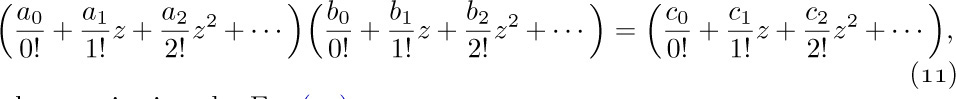
We can then try to obtain information about the function G. This function is a single quantity that represents the whole sequence; if the sequence $\langle{a_{n}}\rangle$ has been defined inductively (that is, if $a_{n}$ has been defined in terms of $a_{0}, a_{1},..., a_{n-1}$) this is an important advantage. Furthermore, we can recover the individual values of a_{0}, a_{1}, ... from the function $G(z)$, assuming that the infinite sum in Eq. (1) exists for some nonzero value of z, by using techniques of differential calculus.

We call $G(z)$ the generating function for the sequence $a_{0}, a_{1}, a_{2},...$. The use of generating functions opens up a whole new range of techniques, and it broadly increases our capacity for problem solving. As mentioned in the previous section, A. de Moivre introduced generating functions in order to solve the general linear recurrence problem. De Moivre’s theory was extended to slightly more complicated recurrences by James Stirling, who showed how to apply differentiation and integration as well as arithmetic operations [Methodus Differentialis (London: 1730), Proposition 15]. A few years later, L. Euler began to use generating functions in several new ways, for example in his papers on partitions [Commentarii Acad. Sci. Pet. 13 (1741), 64–93; Novi Comment. Acad. Sci. Pet. 3 (1750), 125–169]. Pierre S. Laplace developed the techniques further in his classic work Théorie Analytique des Probabilités (Paris: 1812).

The question of convergence of the infinite sum (1) is of some importance. Any textbook about the theory of infinite series will prove that:

a) If the series converges for a particular value of z = z_{0}, then it converges for all values of z with $|z|\lt |z_{0}|$.

b) The series converges for some z ≠ 0 if and only if the sequence

is bounded. (If this condition is not satisfied, we may be able to get a convergent series for the sequence $\langle{a_{n}/n!}\rangle$ or for some other related sequence.)

On the other hand, it often does not pay to worry about convergence of the series when we work with generating functions, since we are only exploring possible approaches to the solution of some problem. When we discover the solution by any means, however sloppy, we may be able to justify the solution independently. For example, in the previous section we used a generating function to deduce Eq. (14); yet once such an equation has been found, it is a simple matter to prove it by induction, and we need not even mention that we used generating functions to discover it. Furthermore one can show that most (if not all) of the operations we do with generating functions can be rigorously justified without regard to the convergence of the series. See, for example, E. T. Bell, Trans. Amer. Math. Soc. 25 (1923), 135–154; Ivan Niven, AMM 76 (1969), 871–889; Peter Henrici, Applied and Computational Complex Analysis 1 (Wiley, 1974), Chapter 1.

A. Addition. If $G(z)$ is the generating function for $\langle{a_{n}}\rangle=a_{0}, a_{1},...$ and $H (z)$ is the generating function for $\langle{b_{n}}\rangle=b_{0}, b_{1},...$, then $αG(z)+βH (z)$ is the generating function for $\langle{αa_{n}+βb_{n}}\rangle=αa_{0}+βb_{0}, αa_{1}+βb_{1},...$:

B. Shifting. If $G(z)$ is the generating function for $\langle{a_{n}}\rangle=a_{0}, a_{1},...$ then $z^{m}G(z)$ is the generating function for $\langle{a_{n-m}}\rangle=0,..., 0, a_{0}, a_{1},...$:

The last summation may be extended over all n ≥ 0 if we regard $a_{n}=0$ for any negative value of n.

Similarly, $(G(z)-a_{0}-a_{1}z-...-a_{m-1}z^{m-1})/z^{m}$ is the generating function for $\langle{a_{n+m}}\rangle=a_{m}, a_{m+1},...$:

We combined operations A and B to solve the Fibonacci problem in the previous section: $G(z)$ was the generating function for $\langle{F_{n}}\rangle$, $z G(z)$ for $\langle{F_{n-1}}\rangle$, $z^{2}G(z)$ for $\langle{F_{n-2}}\rangle$, and $(1-z-z^{2}) G(z) for\langle{F_{n}-F_{n-1}-F_{n-2}}\rangle$. Then, since $F_{n}-F_{n-1}-F_{n-2}$ is zero when n ≥ 2, we found that $(1-z-z^{2})G(z)$ is a polynomial. Similarly, given any linearly recurrent sequence, that is, a sequence where $a_{n}=c_{1}a_{n-1}+···+c_{m}a_{n-m}$, the generating function will be a polynomial divided by $(1-c_{1}z-···-c_{m}z^{m})$.

Let us consider the simplest example of all: If $G(z)$ is the generating function for the constant sequence $1, 1, 1,...$, then $z G(z)$ generates $0, 1, 1,...$, so $(1-z)G(z)=1$. This gives us the simple but very important formula

C. Multiplication. If $G(z)$ is the generating function for $a_{0}, a_{1},...$ and $H (z)$ is the generating function for $b_{0}, b_{1},...$, then

thus $G(z)H (z)$ is the generating function for the sequence $c_{0}, c_{1},...$, where

Equation (3) is a very special case of this. Another important special case occurs when each $b_{n}$ is equal to unity:

The rule for a product of three functions follows from (6); $F (z)G(z)H (z)$ generates $d_{0}, d_{1}, d_{2},...$, where

The general rule for products of any number of functions (whenever this is meaningful) is

When the recurrence relation for some sequence involves binomial coefficients, we often want to get a generating function for a sequence $c_{0}, c_{1},...$ defined by

In this case it is usually better to use generating functions for the sequences $\langle{a_{n}/n!}\rangle$, $\langle{b_{n}/n!}\rangle$, $\langle{c_{n}/n!}\rangle$, since we have

D. Change of z. Clearly $G(cz)$ is the generating function for the sequence $a_{0}, ca_{1}, c_{2}a_{2},...$. As a particular case, the generating function for $1, c, c^{2}, c^{3},...$ is $1/(1-cz)$.

Using complex roots of unity, we can extend this idea and extract every mth term: Let $ω=e^{2πi/m}=\cos(2π/m)+i\sin(2π/m)$; we have

(See exercise 14.) For example, if m = 3 and r = 1, we have

, a complex cube root of unity; it follows that

E. Differentiation and integration. The techniques of calculus give us further operations. If $G(z)$ is given by Eq. (1), the derivative is

The generating function for the sequence $\langle{na_{n}}\rangle$ is $z G′ (z)$. Hence we can combine the nth term of a sequence with polynomials in n by manipulating the generating function.

We can combine the second formula with Eq. (7) to get the generating function for the harmonic numbers:

F. Known generating functions. Whenever it is possible to determine the power series expansion of a function, we have implicitly found the generating function for a particular sequence. These special functions can be quite useful in conjunction with the operations described above. The most important power series expansions are given in the following list.

When r is a negative integer, we get a special case already reflected in Eqs. (5) and (16):

if x is the continuous function of z that solves the equation $x^{t+1}=x^{t}+z$, where x = 1 when z = 0.

Further generalizations, including many sums of harmonic numbers, appear in papers by D. A. Zave, Inf. Proc. Letters 5 (1976), 75–77; J. Spieß, Math. Comp. 55 (1990), 839–863.

The coefficients $B_{k}$ that appear in the last formula are the Bernoulli numbers; they will be examined further in Section 1.2.11.2. A table of Bernoulli numbers appears in Appendix A.

if x is the continuous function of z that solves the equation $x=e^{zx^{t}}$, where x = 1 when z = 0. Significant generalizations of (21) and (30) are discussed in exercise 4.7–22.

for the coefficient of $z^{n}$ in $G(z)$. For example, if $G(z)$ is the generating function in (1) we have $[z^{n}] G(z)=a_{n}$ and

. One of the most fundamental results in the theory of complex variables is a formula of A. L. Cauchy [Exercices de Math. 1 (1826), 95–113 = Œuvres (2) 6, 124–145, Eq. (11)], by which we can extract any desired coefficient with the help of a contour integral:

if $G(z)$ converges for $z=z_{0}$ and $0\lt r\lt |z_{0} |$. The basic idea is that

is zero for all integers m except m = −1, when the integral is

Equation (32) is of importance primarily when we want to study the approximate value of a coefficient.

We conclude this section by returning to a problem that was only partially solved in Section 1.2.3. We saw in Eq. 1.2.3–(13) and exercise 1.2.3–29 that

In general, suppose that we have n numbers $x_{1}, x_{2},..., x^{n}$ and we want the sum

If possible, this sum should be expressed in terms of $S_{1}, S_{2},..., S_{m}$, where

the sum of j th powers. Using this more compact notation, the formulas above become

;

So $G(z)$ is the reciprocal of a polynomial. It often helps to take the logarithm of a product, and we find from (17) that

Now $\ln G(z)$ has been expressed in terms of the S’s; so all we must do to obtain the answer to our problem is to compute the power series expansion of $G(z)$ again, with the help of (22) and (9):

The parenthesized quantity is $h_{m}$. This rather imposing sum is really not complicated when it is examined carefully. The number of terms for a particular value of m is $p(m)$, the number of partitions of m (Section 1.2.1). For example, one partition of 12 is

this corresponds to a solution of the equation $k_{1}+2k_{2}+···+12k_{12}=12$, where $k_{j}$ is the number of j’s in the partition. In our example $k_{1}=1$, $k_{2}=3$, $k_{5}=1$, and the other k’s are zero; so we get the term

as part of the expression for $h_{12}$. By differentiating (37) it is not difficult to derive the recurrence

An enjoyable introduction to the applications of generating functions has been given by G. Pólya, “On picture writing,” AMM 63 (1956), 689–697; his approach is continued in CMath, Chapter 7. See also the book generatingfunctionology by H. S. Wilf, second edition (Academic Press, 1994). 94

A generating function is a clothesline
on which we hang up a sequence of numbers for display.

1. [M12] What is the generating function for the sequence $2, 5, 13, 35,...=\langle{2^{n} +3^{n}}\rangle$?

3. [HM21] Differentiate the generating function (18) for $\langle{H_{n}}\rangle$, and compare this with the generating function for

. What relation can you deduce?

8. [M23] Find the generating function for $p(n)$, the number of partitions of n.

9. [M11] In the notation of Eqs. (34) and (35), what is $h_{4}$ in terms of $S_{1}$, $S_{2}$, $S_{3}$, and $S_{4}$?

(This is the same as $h_{m}$ of Eq. (33), except that equal subscripts are not allowed.) Find the generating function for $e_{m}$, and express $e_{m}$ in terms of the $S_{j}$ in Eq. (34). Write out the formulas for $e_{1}$, $e_{2}$, $e_{3}$, and $e_{4}$.

11. [M25] Equation (39) can also be used to express the S’s in terms of the h’s: We find $S_{1}=h_{1}$,

, etc. What is the coefficient of

in this representation of $S_{m}$, when $k_{1}+2k_{2}+···+mk_{m}=m$?

12. [M20] Suppose we have a doubly subscripted sequence $\langle{a_{mn}}\rangle$ for $m, n=0, 1,...$; show how this double sequence can be represented by a single generating function of two variables, and determine the generating function for

Given that $a_{0}, a_{1}, a_{2},...$ is an infinite sequence having a convergent generating function, let $f(x)$ be the step function $∑_{k}a_{k}[0≤k≤x]$. Express the Laplace transform of $f(x)$ in terms of the generating function G for this sequence.

15. [M28] By considering $H (w)=∑_{n≥0}G_{n}(z)w^{n}$, find a closed form for the generating function

16. [M22] Give a simple formula for the generating function $G_{nr}(z)=∑_{k}a_{nkr} z^{k}$, where $a_{nkr}$ is the number of ways to choose k out of n objects, subject to the condition that each object may be chosen at most r times. (If r = 1, we have

ways, and if r ≥ k, we have the number of combinations with repetitions as in exercise 1.2.6–60.)

17. [M25] What are the coefficients of $1/(1-z)^{w}$ if this function is expanded into a double power series in terms of both z and w?

18. [M25] Given positive integers n and r, find a simple formula for the value of the following sums: (a) $∑_{1≤k_{1}\lt k_{2}\lt...\lt k_{r}≤n}k_{1}k_{2}... k_{r}$; (b) $∑_{1≤k_{1}≤k_{2}≤k_{r}≤n}k_{1}k_{2}... k_{r}$. (For example, when n = 3 and r = 2 the sums are, respectively, $1·2+1·3+2·3$ and $1·1+1·2+1·3+2·2+2·3+3·3$.)

19. [HM32] (C. F. Gauss, 1812.) The sums of the following infinite series are well known:

found in the answer to exercise 1.2.7–24, these series may be written respectively as

when p and q are integers with 0 < p < q. [Hint: By Abel’s limit theorem the sum is

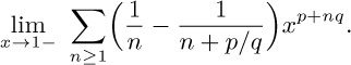
Use Eq. (13) to express this power series in such a way that the limit can be evaluated.]

21. [HM30] Set up the generating function for the sequence $\langle{n!}\rangle$ and study properties of this function.

23. [M33] (L. Carlitz.) (a) Prove that for all integers m ≥ 1 there are polynomials $f_{m}(z_{1},..., z_{m})$ and $g_{m}(z_{1},..., z_{m})$ such that the formula

Evaluate both sides of this identity when $G(z)$ is (a) $1/(1-z)$; (b) $(e^{z}-1)/z$.

25. [M23] Evaluate the sum

by simplifying the equivalent formula $∑_{k}[w^{k}] (1-2w)^{n}[z^{n-k}] (1+z)^{2n-2k}$.

26. [M40] Explore a generalization of the notation (31) according to which we might write, for example, $[z^{2}-2z^{5}] G(z)=a_{2}-2a_{5}$ when $G(z)$ is given by (1).

1.2.10. Analysis of an Algorithm

Let us now apply some of the techniques of the preceding sections to the study of a typical algorithm.

Algorithm M (Find the maximum). Given n elements $X[1], X[2],..., X[n]$, we will find m and j such that $m=X[j]=\max_{1≤i≤n}X[i]$, where j is the largest index that satisfies this relation.

M1. [Initialize.] Set $j←n$, $k←n-1$, $m←x[n]$. (During this algorithm we will have $m=X[j]=\max_{k\lt i≤n}X[i]$.)

M4. [Change m.] Set $j←k$, $m←X[k]$. (This value of m is a new current maximum.)

This rather obvious algorithm may seem so trivial that we shouldn’t bother to analyze it in detail; but it actually makes a good demonstration of the way in which more complicated algorithms may be studied. Analysis of algorithms is quite important in computer programming, because there are usually several algorithms available for a particular application and we would like to know which is best.

Algorithm M requires a fixed amount of storage, so we will analyze only the time required to perform it. To do this, we will count the number of times each step is executed (see Fig. 9):

Fig. 9. Algorithm M. Labels on the arrows indicate the number of times each path is taken. Note that “Kirchhoff’s first law” must be satisfied: The amount of flow into each node must equal the amount of flow going out.

Knowing the number of times each step is executed gives us the information necessary to determine the running time on a particular computer.

In the table above we know everything except the quantity A, which is the number of times we must change the value of the current maximum. To complete the analysis, we shall study this interesting quantity A.

The analysis usually consists of finding the minimum value of A (for optimistic people), the maximum value of A (for pessimistic people), the average value of A (for probabilistic people), and the standard deviation of A (a quantitative indication of how close to the average we may expect the value to be).

Thus the average value lies between 0 and $n-1$. Is it

n? Is it

? To answer this question we need to define what we mean by the average; and to define the average properly, we must make some assumptions about the characteristics of the input data $X[1], x[2],..., x[n]$. We will assume that the $X[k]$ are distinct values, and that each of the n! permutations of these values is equally likely. (This is a reasonable assumption to make in most situations, but the analysis can be carried out under other assumptions, as shown in the exercises at the end of this section.)

The performance of Algorithm M does not depend on the precise values of the X [k]; only the relative order is involved. For example, if n = 3 we are assuming that each of the following six possibilities is equally probable:

It is clear that we may take $X[1], X[2],..., X[n]$ to be the numbers $1, 2,..., n$ in some order; under our assumption we regard each of the $n!$ permutations as equally likely. The probability that A has the value k will be

The variance $V_{n}$ is defined to be the average value of $(A-A_{n})^{2}$; we have therefore

The significance of $σ_{n}$ can perhaps best be understood by noting that, for all r ≥ 1, the probability that A fails to lie within $rσ_{n}$ of its average value is less than $1/r^{2}$. For example, $|A-A_{n} |\gt2σ_{n}$ with probability < 1/4. (Proof: Let p be the stated probability. Then if p > 0, the average value of $(A-A_{n}) ^{2}$ is more than $p·(rσ_{n})^{2}+(1-p)·0$; that is, $V_{n}\gt pr^{2}V_{n}$.) This is usually called Chebyshev’s inequality, although it was actually discovered first by J. Bienaymé [Comptes Rendus Acad. Sci. 37 (Paris, 1853), 320–321].

We can determine the behavior of A by determining the probabilities $p^{nk}$. It is not hard to do this inductively: By Eq. (1) we want to count the number of permutations on n elements that have A = k. Let this number be $p_{nk}=n! p_{nk}$.

Consider the permutations $x_{1}x_{2}... x_{n}$ on $/{1, 2,..., n/}$, as in Section 1.2.5. If $x_{1}=n$, the value of A is one higher than the value obtained on $x_{2}... x^{n}$; if $x_{1} ≠ n$, the value of A is exactly the same as its value on $x_{2}... x_{n}$. Therefore we find that $p_{nk}=P_(n-1)(k-1)+(n-1)P_{(n-1) k}$, or equivalently

Fig. 10. Probability distribution for step M4, when n = 12. The mean is $58301/27720$, or approximately 2.10. The variance is approximately 1.54.

We can now get information about the quantities Pnk by using generating functions. Let

We know that A ≤ n – 1, so $p_{nk}= 0$ for large values of k; thus $G_{n}(z)$ is actually a polynomial, even though an infinite sum has been specified for convenience.

(The reader should study the relation between Eqs. (4) and (7) carefully.) We can now see that

Now all we must do is plug this value of p_nk into Eqs. (2) and (3) and we have the desired average value. But this is easier said than done. It is, in fact, unusual to be able to determine the probabilities $p_{nk}$ explicitly; in most problems we will know the generating function $G_{n}(z)$, but we will not have any special knowledge about the actual probabilities. The important fact is that we can determine the mean and variance easily from the generating function itself.

To see this, let’s suppose that we have a generating function whose coefficients represent probabilities:

Here $p_{k}$ is the probability that some event has a value k. We wish to calculate the quantities

since $G(1)=p_{0}+p_{1}+p_{2}+···$ is the sum of all possible probabilities. Similarly, since $G′(z)=∑_{k}kp_{k}z^{k-1}$, we have

Equations (12) and (13) give the desired expressions of the mean and variance in terms of the generating function.

This is the desired average number of times step M4 is executed; it is approximately ln n when n is large. [Note: The rth moment of $A+1$, namely the quantity $∑_{k}(k+1)^{r}p_{nk}$, is

, and it has the approximate value $(\ln n)^{r}$; see P. B. M. Roes CACM 9 (1966), 342. The distribution of A was first studied by F. G. Foster and A. Stuart, J. Roy. Stat. Soc. B16 (1954), 1–22.]

We can proceed similarly to calculate the variance $V_{n}$. Before doing this, let us state an important simplification:

Theorem A. Let G and H be two generating functions with $G(1)=H (1)=1$. If the quantities ${\rm mean}(G)$ and ${\rm var}(G)$ are defined by Eqs. (12) and (13), we have

We will prove this theorem later. It tells us that the mean and variance of a product of generating functions may be reduced to a sum.

The notation used in Eq. (16) will be used to describe the statistical characteristics of other probabilistic quantities throughout this book.

We have completed the analysis of Algorithm M; the new feature that has appeared in this analysis is the introduction of probability theory. Elementary probability theory is sufficient for most of the applications in this book: The simple counting techniques and the definitions of mean, variance, and standard deviation already given will answer most of the questions we want to ask. More complicated algorithms will help us develop an ability to reason fluently about probabilities.

Let us consider some simple probability problems, to get a little more practice using these methods. In all probability the first question that comes to mind is a coin-tossing problem: Suppose we flip a coin n times and there is a probability p that heads turns up after any particular toss; what is the average number of heads that will occur? What is the standard deviation?

We will consider our coin to be biased; that is, we will not assume that p =

. This makes the problem more interesting, and, furthermore, every real coin is biased (or we could not tell one side from the other).

Proceeding as before, we let $p_{nk}$ be the probability that k heads will occur, and let $G_{n}(z)$ be the corresponding generating function. We have clearly

where $q=1-p$ is the probability that tails turns up. As before, we argue from Eq. (17) that $G_{n}(z)=(q+pz)G_{n-1}(z)$; and from the obvious initial condition $G_{1}(z)=q+pz$ we have

Figure 11 shows the values of $p_{nk}$ when

, n = 12. When the standard deviation is proportional to

and the difference between maximum and minimum is proportional to n, we may consider the situation “stable” about the average.

Fig. 11. Probability distribution for coin-tossing: 12 independent tosses with a chance of success equal to 3/5 at each toss.

Let us work one more simple problem. Suppose that in some process there is equal probability of obtaining the values $1, 2,..., n$. The generating function for this situation is

Now to calculate the mean and variance, we need to know G′(1) and $G″(1)$; but the form in which we have expressed these equations reduces to $0/0$ when we substitute z = 1. This makes it necessary to find the limit as z approaches unity, and that is a nontrivial task.

Fortunately there is a much simpler way to proceed. By Taylor’s theorem we have

therefore we merely have to replace z by z + 1 in (20) and read off the coefficients:

In this case the deviation of approximately $0.289n$ gives us a recognizably unstable situation.

We conclude this section by proving Theorem A and relating our notions to classical probability theory. Suppose X is a random variable that takes on only nonnegative integer values, where X = k with probability $p_{k}$. Then $G(z)=p_{0}+p_{1}z+p_{2}z^{2}+···$ is called the probability generating function for X, and the quantity $G(e^{it})=p_{0} +p_{1} e^{it} +p_{2}e^{2it} +···$ is conventionally called the characteristic function of this distribution. The distribution given by the product of two such generating functions is called the convolution of the two distributions, and it represents the sum of two independent random variables belonging to those respective distributions.

The mean or average value of a random quantity X is often called its expected value, and denoted by ${\rm E}X$. The variance of X is then ${\rm E}X^{2}-({\rm E}X)^{2}$. Using this notation, the probability generating function for X is $G(z)={\rm E}z^{X}$, the expected value of $z^{X}$, in cases when X takes only nonnegative integer values. Similarly, if X is a statement that is either true or false, the probability that X is true is $\Pr(X)={\rm E}[X ]$, using Iverson’s convention (Eq. 1.2.3–(16)).

The mean and variance are just two of the so-called semi-invariants or cumulants introduced by T. N. Thiele in 1889 [see A. Hald, International Statistical Review 68 (2000), 137–153]. The semi-invariants $κ_{1}, κ_{2}, κ_{3},...$ are defined by the rule

Since the semi-invariants are defined in terms of the logarithm of a generating function, Theorem A is obvious, and, in fact, it can be generalized to apply to all of the semi-invariants.

A normal distribution is one for which all semi-invariants are zero except the mean and variance. In a normal distribution, we can improve significantly on Chebyshev’s inequality: The probability that a normally distributed random value differs from the mean by less than the standard deviation is

that is, about $68.268949213709\%$ of the time. The difference is less than twice the standard deviation about $95.449973610364\%$ of the time, and it is less than three times the standard deviation about $99.730020393674\%$ of the time. The distributions specified by Eqs. (8) and (18) are approximately normal when n is large (see exercises 13 and 14).

We often need to know that a random variable is unlikely to be much larger or smaller than its mean value. Two extremely simple yet powerful formulas, called the tail inequalities, provide convenient estimates of such probabilities. If X has the probability generating function $G(z)$, then

$\Pr(X≤r)=p_{0}+p_{1}+···+p_{\lfloor{r}\rfloor}≤x^{-r}p_{0}+x^{1-r}p_{1}+···+x^{\lfloor{r}\rfloor-r}p_{\lfloor{r}\rfloor}≤x^{-r}G(x)$

$\Pr(X ≥ r)=p_{\lceil{r}\rceil}+p_{\lceil{r}\rceil+1}+···≤x^{\lceil{r}\rceil-r}p_{\lceil{r}\rceil}+x^{\lceil{r}\rceil+1-r}p_{\lceil{r}\rceil+1}+···≤x^{-r}G(x)$

when x ≥ 1. By choosing values of x that minimize or approximately minimize the right-hand sides of (24) and (25), we often obtain upper bounds that are fairly close to the true tail probabilities on the left-hand sides.

Exercises 21–23 illustrate the tail inequalities in several important cases. These inequalities are special cases of a general principle pointed out by A. N. Kolmogorov in his book Grundbegriffe der Wahrscheinlichkeitsrechnung (1933): If $f(t) ≥ s\gt0$ for all t ≥ r, and if $f(t) ≥ 0$ for all t in the domain of the random variable X, then $\Pr(X ≥ r)≤s^{-1} {\rm E}f(X)$ whenever ${\rm E}f(X)$ exists. We obtain (25) when $f(t)=x^{t}$ and $s=x^{r}$. [S. Bernstein had contributed key ideas in Uchenye zapiski Nauchno-Issledovatel’skikh kafedr Ukrainy 1 (1924), 38–48.]

1. [10] Determine the value of $p_n0$ from Eqs. (4) and (5) and interpret this result from the standpoint of Algorithm M.

3. [M15] What are the minimum, maximum, average, and standard deviation of the number of times step M4 is executed, if we are using Algorithm M to find the maximum of 1000 randomly ordered, distinct items? (Give your answer as decimal approximations to these quantities.)

4. [M10] Give an explicit, closed formula for the values of p_nk in the coin-tossing experiment, Eq. (17).

5. [M13] What are the mean and standard deviation of the distribution in Fig. 11?

6. [HM27] We’ve computed the mean and the variance of the important probability distributions (8), (18), (20). What is the third semi-invariant, $k_{3}$, in each of those cases?

7. [M27] In our analysis of Algorithm M, we assumed that all the $X[k]$ were distinct. Suppose, instead, that we make only the weaker assumption that $X[1], X[2],..., X[n]$ contain precisely m distinct values; the values are otherwise random, subject to this constraint. What is the probability distribution of A in this case?

8. [M20] Suppose that each $X[k]$ is taken at random from a set of M distinct elements, so that each of the $M ^{n}$ possible choices for $X[1], X[2],..., X[n]$ is considered equally likely. What is the probability that all the $X[k]$ will be distinct?

9. [M25] Generalize the result of the preceding exercise to find a formula for the probability that exactly m distinct values occur among the X’s. Express your answer in terms of Stirling numbers.

10. [M20] Combine the results of the preceding three exercises to obtain a formula for the probability that A = k under the assumption that each X is selected at random from a set of M objects.

11. [M15] What happens to the semi-invariants of a distribution if we change $G(z)$ to $F (z)=z^{n}G(z)$?

12. [HM21] When $G(z)=p_{0}+p_{1}z+p_{2}z^{2}+···$ represents a probability distribution, the quantities $M_{n}=∑_{k}k^{n}p_{k}$ and $m_{n}=∑_{k} (k-M_{1}) ^{n}p_{k}$ are called the “nth moment” and “nth central moment,” respectively. Show that $G(e^{t})=1+M_{1}t+M_{2}t^{2}/2!+...$; then use Arbogast’s formula (exercise 1.2.5–21) to show that

In particular, $κ_{1}=M_{1}$,

(as we already knew),

, and

. What are the analogous expressions for $κ_{n}$ in terms of the central moments $m_{2}, m_{3},...$, when n ≥ 2?

13. [HM38] A sequence of probability generating functions $G_{n}(z)$ with means $μ_{n}$ and deviations $σ_{n}$ is said to approach a normal distribution if

for all real values of t. Using $G_{n}(z)$ as given by Eq. (8), show that $G_{n}(z)$ approaches a normal distribution.

Note: “Approaching the normal distribution,” as defined here, can be shown to be equivalent to the fact that

where $X_{n}$ is a random quantity whose probabilities are specified by $G_{n}(z)$. This is a special case of P. Lévy’s important “continuity theorem,” a basic result in mathematical probability theory. A proof of Lévy’s theorem would take us rather far afield, although it is not extremely difficult [for example, see Limit Distributions for Sums of Independent Random Variables by B. V. Gnedenko and A. N. Kolmogorov, translated by K. L. Chung (Reading, Mass.: Addison–Wesley, 1954)].

14. [HM30] (A. de Moivre.) Using the conventions of the previous exercise, show that the binomial distribution $G_{n}(z)$ given by Eq. (18) approaches the normal distribution.

15. [HM23] When the probability that some quantity has the value k is $e^{-μ} (μ^{k}/k!)$, it is said to have the Poisson distribution with mean μ.

c) Show that as $n → ∞$ the Poisson distribution with mean np approaches the normal distribution in the sense of exercise 13.

16. [M25] Suppose X is a random variable whose values are a mixture of the probability distributions generated by $g_{1}(z), g_{2}(z),..., g_{r}(z)$, in the sense that it uses $g_{k}(z)$ with probability $p_{k}$, where $p_{1}+p_{2}+···+p_{r}=1$. What is the generating function for X? Express the mean and variance of X in terms of the means and variances of $g_{1}, g_{2},..., g_{r}$.

17. [M27] Let f (z) and $g(z)$ be generating functions that represent probability distributions.

a) Show that $h(z)=g(f(z))$ is also a generating function representing a probability distribution.

b) Interpret the significance of $h(z)$ in terms of $f(z)$ and $g(z)$. (What is the meaning of the probabilities represented by the coefficients of $h(z)$?)

18. [M28] Suppose that the values taken on by $X[1], X[2],..., X[n]$ in Algorithm M include exactly $k_{1}$ ones, $k_{2}$ twos, ..., $k_{n}$ n’s, arranged in random order. (Here

The assumption in the text is that $k_{1}=k_{2}=···= k_{n}=1$.) Show that in this generalized situation, the generating function (8) becomes

19. [M21] If a_{k} > a_{j} for 1 ≤ j < k, we say that a_{k} is a left-to-right maximum of the sequence a_{1}a_{2} ... a_{n}. Suppose a_{1}a_{2} ... a_{n} is a permutation of {1, 2, ..., n}, and let b_{1}b_{2} ... b_{n} be the inverse permutation, so that a_{k} = l if and only if b_{l} = k. Show that a_{k} is a left-to-right maximum of a₁ a₂ ... a_n if and only if k is a right-to-left minimum of b_{1}b_{2} ... b_{n}.

20. [M22] Suppose we want to calculate max{|a_{1} − b_{1} |, |a_{2} − b_{2} |, ..., |a_{n} − b_{n} |} when b_{1} ≤ b_{2} ≤ · · · ≤ b_{n}. Show that it is sufficient to calculate max{m_L, m_R }, where

m_L = max{a_k − b_k | a_k is a left-to-right maximum of a_{1}a_{2} ... a_{n} },

m_R = max{b_k − a_k | a_k is a right-to-left minimum of a_{1}a_{2} ... a_{n} } .

(Thus, if the a’s are in random order, the number of k’s for which a subtraction must be performed is only about 2 ln n.)

21. [HM21] Let X be the number of heads that occur when a random coin is flipped n times, with generating function (18). Use (25) to prove that

22. [HM22] Suppose X has the generating function (q_{1} + p_{1}z)(q_{2} + p_{2}z) ... (q_{n} + p_{n}z), where p_{k} + q_{k} = 1 for 1 ≤ k ≤ n. Let μ = {\rm E}X = p_{1} + p_{2} + · · · + p_{n}. (a) Prove that

Pr(X ≤ μr) ≤ (r^−r e^r−1) ^μ, when 0 < r ≤ 1;
Pr(X ≥ μr) ≤ (r^−r e^r−1) ^μ, when r ≥ 1.

(b) Express the right-hand sides of these estimates in convenient form when r ≈ 1.

23. [HM23] Estimate the tail probabilities for a random variable that has the negative binomial distribution generated by (q − pz)⁻ⁿ, where q = p + 1.

*1.2.11. Asymptotic Representations

We often want to know a quantity approximately, instead of exactly, in order to compare it to another. For example, Stirling’s approximation to n! is a useful representation of this type, when n is large, and we have also made use of the fact that $H_{n}≈\ln n+γ$. The derivations of such asymptotic formulas generally involve higher mathematics, although in the following subsections we will use nothing more than elementary calculus to get the results we need.

*1.2.11.1. The $O$-notation

Paul Bachmann introduced a very convenient notation for approximations in his book Analytische Zahlentheorie (1894). It is the O-notation, which allows us to replace the “≈” sign by “=” and to quantify the degree of accuracy; for example,

(Read, “H sub n equals the natural log of n plus Euler’s constant [pronounced ‘Oiler’s constant’] plus big-oh of one over n.”)

In general, the notation O(f (n)) may be used whenever f (n) is a function of the positive integer n; it stands for a quantity that is not explicitly known, except that its magnitude isn’t too large. Every appearance of O(f (n)) means precisely this: There are positive constants M and n_{0} such that the number x_{n} represented by O(f (n)) satisfies the condition |x_n | ≤ M |f(n)|, for all integers n ≥ n_{0}. We do not say what the constants M and n_{0} are, and indeed those constants are usually different for each appearance of O.

For example, Eq. (1) means that |H_{n} − ln n − γ| ≤ M/n when n ≥ n_{0}. Although the constants M and n_{0} are not stated, we can be sure that the quantity O(1/n) will be arbitrarily small if n is large enough.

Equation (2) is rather crude, but not incorrect; Eq. (3) is a stronger statement; and Eq. (4) is stronger yet. To justify these equations we shall prove that if P (n) = a_{0} + a_{1}n + · · · + a_{m}n^{m}is any polynomial of degree m or less, then we have P (n) = O(n^{m}). This follows because

when n ≥ 1. So we may take M = |a_{0}| + |a_{1}| + · · · + |a_{m}| and n_{0} = 1. Or we could take, say, M = |a_{0}|/2^m + |a_{1}|/2^m−1 + · · · + |a_{m}| and n_{0} = 2.

The O-notation is a big help in approximation work, since it describes briefly a concept that occurs often and it suppresses detailed information that is usually irrelevant. Furthermore, it can be manipulated algebraically in familiar ways, although certain important differences need to be kept in mind. The most important consideration is the idea of one-way equalities: We write

, but we never write

. (Or else, since

, we might come up with the absurd relation

.) We always use the convention that the right-hand side of an equation does not give more information than the left-hand side; the right-hand side is a “crudification” of the left.

This convention about the use of “=” may be stated more precisely as follows: Formulas that involve the O(f (n))-notation may be regarded as sets of functions of n. The symbol O(f (n)) stands for the set of all functions g of integers such that there exist constants M and n_{0} with |g(n)| ≤ M |f(n)| for all integers n ≥ n_{0}. If S and T are sets of functions, then S + T denotes the set \{g + h | g ∊ S and h ∊ T\}; we define S + c, S − T, S · T, log S, etc., in a similar way. If $α(n)$ and $β(n)$ are formulas that involve the O-notation, then the notation α(n) = β(n) means that the set of functions denoted by $α(n)$ is contained in the set denoted by $β(n)$.

Consequently we may perform most of the operations we are accustomed to doing with the “=” sign: If α(n) = β(n) and β(n) = γ(n), then α(n) = γ(n). Also, if α(n) = β(n) and if δ(n) is a formula resulting from the substitution of β(n) for some occurrence of α(n) in a formula γ(n), then γ(n) = δ(n). These two statements imply, for example, that if g(x_{1}, x_{2}, ..., x_{m}) is any real function whatever, and if α_{k} (n) = β_{k} (n) for 1 ≤ k ≤ m, then g(α_{1} (n), α_{2} (n), ..., α_{m} (n)) = g(β_{1} (n), β_{2} (n), ..., β_{m} (n)).

The O-notation is also frequently used with functions of a complex variable z, in the neighborhood of z = 0. We write O(f (z)) to stand for any quantity g(z) such that |g(z)| ≤ M |f(z)| whenever |z| < r. (As before, M and r are unspecified constants, although we could specify them if we wanted to.) The context of O-notation should always identify the variable that is involved and the range of that variable. When the variable is called n, we implicitly assume that O(f (n)) refers to functions of a large integer n; when the variable is called z, we implicitly assume that O(f (z)) refers to functions of a small complex number z.

that converges for z = z_{0}. Then the sum of absolute values ∑_k≥0 |a_k z^k| also converges whenever |z| < |z_{0} |. If z_{0} ≠ 0, we can therefore always write

For we have g(z) = a_{0} + a_{1}z + · · · + a_{m}z^{m} + z^{m + 1} (a_{m + 1} + a_{m + 2}z + · · ·); we need only show that the parenthesized quantity is bounded when |z| ≤ r, for some positive r, and it is easy to see that |a_{m + 1}| + |a_{m + 2}| r + |a_{m + 3}| r^{2} + · · · is an upper bound whenever |z| ≤ r < |z_{0}|.

For example, the generating functions listed in Section 1.2.9 give us many important asymptotic formulas valid when z is sufficiently small, including

for all nonnegative integers m. It is important to note that the hidden constants M and r implied by any particular O are related to each other. For example, the function e^z is obviously O(1) when |z| ≤ r, for any fixed r, since |e^{z} | ≤ e^|z|; but there is no constant M such that |e^z | ≤ M for all values of z. Therefore we need to use larger and larger bounds M as the range r increases.

Sometimes an asymptotic series is correct although it does not correspond to a convergent infinite series. For example, the basic formulas that express factorial powers in terms of ordinary powers,

are asymptotically valid for any real r and any fixed integer m ≥ 0, yet the sum

diverges for all n. (See exercise 12.) Of course, when r is a nonnegative integer,

and

are simply polynomials of degree r, and (17) is essentially the same as 1.2.6–(44). When r is a negative integer and |n| > |r|, the infinite sum

does converge to

; this sum can also be written in the more natural form

, using Eq. 1.2.6–(58).

Let us give one simple example of the concepts we have introduced so far. Consider the quantity

; as n gets large, the operation of taking an nth root tends to decrease the value, but it is not immediately obvious whether

decreases or increases. It turns out that

decreases to unity. Let us consider the slightly more complicated quantity

. Now

gets smaller as n gets bigger; what happens to

because ln n/n → 0 as n → ∞; see exercises 8 and 11. This equation proves our previous contention that

→ 1. Furthermore, it tells us that

In other words,

is approximately equal to ln n; the difference is O((ln n)²/n), which approaches zero as n approaches infinity.

People often abuse O-notation by assuming that it gives an exact order of growth; they use it as if it specifies a lower bound as well as an upper bound. For example, an algorithm to sort n numbers might be called inefficient “because its running time is O(n^{2}).” But a running time of O(n^{2}) does not necessarily imply that the running time is not also O(n). There’s another notation, Big Omega, for lower bounds: The statement

Using this notation we can correctly conclude that a sorting algorithm whose running time is Ω(n^{2}) will not be as efficient as one whose running time is O(n log n), if n is large enough. However, without knowing the constant factors implied by O and Ω, we cannot say anything about how large n must be before the O(n log n) method will begin to win.

Finally, if we want to state an exact order of growth without being precise about constant factors, we can use Big Theta: