
1. ${\tt INFO(T)}=A$, ${\tt INFO(RLINK(T))}=C$, etc.; the answer is H.
2. Preorder: 1245367; symmetric order: 4251637; postorder: 4526731.
3. The statement is true; notice, for example, that nodes 4, 5, 6, 7 always appear in this order in exercise 2. The result is immediately proved by induction on the size of the binary tree.
4. It is the reverse of postorder. (This is easily proved by induction.)
5. In the tree of exercise 2, for example, preorder is 1, 10, 100, 101, 11, 110, 111, using binary notation (which is in this case equivalent to the Dewey system). The strings of digits have been sorted, like words in a dictionary.
In general, the nodes will be listed in preorder if they are sorted lexicographically from left to right, with “blank” < 0 < 1. The nodes will be listed in postorder if they are sorted lexicographically with 0 < 1 < “blank”. For inorder, use 0 < “blank” < 1.
(Moreover, if we imagine the blanks at the left and treat the Dewey labels as ordinary binary numbers, we get level order; see 2.3.3–(8).)
6. The fact that $p_{1}p_{2}\ldots p_{n}$ is obtainable with a stack is readily proved by induction on n, or in fact we may observe that Algorithm T does precisely what is required in its stack actions. (The corresponding sequence of S’s and X’s, as in exercise 2.2.1–3, is the same as the sequence of 1s and 2s as subscripts in double order; see exercise 18.)
Conversely, if $p_{1}p_{2}\ldots p_{n}$ is obtainable with a stack and if $p_{k}=1$, then $p_{1}\ldots p_{k-1}$ is a permutation of $\{2,\ldots,k\}$ and $p_{k+1}\ldots p_{n}$ is a permutation of $\{k+1,\ldots,n\}$; these are the permutations corresponding to the left and right subtrees, and both are obtainable with a stack. The proof now proceeds by induction.
7. From the preorder, the root is known; then from the inorder, we know the left subtree and the right subtree; and in fact we know the preorder and inorder of the nodes in the latter subtrees. Hence the tree is readily constructed (and indeed it is quite amusing to construct a simple algorithm that links the tree together in the normal fashion, starting with the nodes linked together in preorder in LLINK and in inorder in RLINK). Similarly, postorder and inorder together characterize the structure. But preorder and postorder do not; there are two binary trees having $AB$ as preorder and $BA$ as postorder. If all nonterminal nodes of a binary tree have both branches nonempty, its structure is characterized by preorder and postorder.
8. (a) Binary trees with all $\tt LLINK\rm s$ null. (b) Binary trees with zero or one nodes. (c) Binary trees with all $\tt RLINK\rm s$ null.
9. T1 once, T2 $2n{+}1$ times, T3 n times, T4 $n{+}1$ times, T5 n times. These counts can be derived by induction or by Kirchhoff’s law, or by examining Program T.
10. A binary tree with all $\tt RLINK\rm s$ null will cause all n node addresses to be put in the stack before any are removed.
11. Let $a_{nk}$ be the number of binary trees with n nodes for which the stack in Algorithm T never contains more than k items. If $g_{k}(z)=∑_{n}a_{nk}z^{n}$, we find $g_{1}(z)=1/(1-z)$, $g_{2}(z)=1/(1-z/(1-z))=$ $(1-z)/(1-2z),\ldots,g_{k}(z)=$ $1/(1-zg_{k-1}(z))=q_{k-1}(z)/q_{k}(z)$ where $q_{-1}(z)=q_{0}(z)=1$, $q_{k+1}(z)=q_{k}(z)-zq_{k-1}(z)$; hence $g_{k}(z)=(f_{1}(z)^{k+1}-f_{2}(z)^{k+1})/(f_{1}(z)^{k+2}-f_{2}(z)^{k+2})$ where $f_{j}(z)=\frac{1}{2}(1\pm\sqrt{1-4z})$. It can now be shown that $a_{nk}=[u^{n}](1-u)(1+u)^{2n}(1-u^{k+1})/(1-u^{k+2})$; hence $s_{n}=∑_{k\ge1}k(a_{nk}-a_{n(k-1)})$ is $[u^{n+1}](1-u)^{2}(1+u)^{2n}∑_{j\ge1}u^{j}/(1-u^{j})$, minus $a_{nn}$. The technique of exercise 5.2.2–52 now yields the asymptotic series
$s_{n}/a_{nn}=\sqrt{\pi n}-\frac{3}{2}-\frac{13}{24}\sqrt{\frac{\pi}{n}}+\frac{1}{2n}+O(n^{-3/2})$
[N. G. de Bruijn, D. E. Knuth, and S. O. Rice, in Graph Theory and Computing, ed. by R. C. Read (New York: Academic Press, 1972), 15–22.]
When the binary tree represents a forest as described in Section 2.3.2, the quantity analyzed here is the height of that forest (the furthest distance between a node and a root, plus one). Generalizations to many other varieties of trees have been obtained by Flajolet and Odlyzko [j. Computer and System Sci. 25 (1982), 171–213]; the asymptotic distribution of heights, both near the mean and far away, was subsequently analyzed by Flajolet, Gao, Odlyzko, and Richmond [Combinatorics, Probability, and Computing 2 (1993), 145–156].
12. Visit $\tt NODE(P)$ between steps T2 and T3, instead of in step T5. For the proof, demonstrate the validity of the statement “Starting at step T2 with $\ldots$ original value ${\tt A[}1{\tt]\ldots A[}m\tt]$,” essentially as in the text.
13. (Solution by S. Araújo, 1976.) Let steps T1 through T4 be unchanged, except that a new variable Q is initialized to Λ in step T1′; Q will point to the last node visited, if any. Step T5 becomes two steps:
T5′. [Right branch done?] If ${\tt RLINK(P)}=\varLambda$ or ${\tt RLINK(P)}=\tt Q$, go on to T6; otherwise set $\tt A\Leftarrow P$, $\tt P←RLINK(P)$ and return to T2′.
T6′. [Visit P.] Visit $\tt NODE(P)$, set $\tt Q←P$, and return to T4′.
A similar proof applies. (Steps T4′ and T5′ can be streamlined so that nodes are not taken off the stack and immediately reinserted.)
14. By induction, there are always exactly n + 1 Λ links (counting T when it is null). There are n nonnull links, counting T, so the remark in the text about the majority of null links is justified.
15. There is a thread LLINK or RLINK pointing to a node if and only if it has a nonempty right or left subtree, respectively. (See Fig. 24.)
16. If ${\tt LTAG(Q)}=0$, Q* is $\tt LLINK(Q)$; thus Q* is one step down and to the left. Otherwise Q* is obtained by going upwards in the tree (if necessary) repeatedly until the first time it is possible to go down to the right without retracing steps; typical examples are the trips from P to P* and from Q to Q* in the following tree:
17. If ${\tt LTAG(P)}=0$, set $\tt Q←LLINK(P)$ and terminate. Otherwise set $\tt Q←P$, then set $\tt Q←RLINK(Q)$ zero or more times until finding ${\tt RTAG(Q)}=0$; finally set $\tt Q←RLINK(Q)$ once more.
18. Modify Algorithm T by inserting a step T2.5, “Visit $\tt NODE(P)$ the first time”; in step T5, we are visiting $\tt NODE(P)$ the second time.
Given a threaded tree the traversal is extremely simple:
$({\tt P},1)^\varDelta=({\tt LLINK(P)},1)$ if ${\tt LTAG(P)}=0$, otherwise $({\tt P},2)$;
$({\tt P},2)^\varDelta=({\tt RLINK(P)},1)$ if ${\tt RTAG(P)}=0$, otherwise $({\tt RLINK(P)},2)$.
In each case, we move at most one step in the tree; in practice, therefore, double order and the values of d and e are embedded in a program and not explicitly mentioned.
Suppressing all the first visits gives us precisely Algorithms T and S; suppressing all the second visits gives us the solutions to exercises 12 and 17.
19. The basic idea is to start by finding the parent Q of P. Then if $\tt P\neq LLINK(Q)$ we have ${\tt P\sharp}=\tt Q$; otherwise we can find $\tt P\sharp$ by repeatedly setting $\tt Q←Q\$$ zero or more times until ${\tt RTAG(Q)}=1$. (See, for example, P and $\tt P\sharp$ in the tree shown.)

There is no efficient algorithm to find the parent of P in a general right-threaded tree, since a degenerate right-threaded tree in which all left links are null is essentially a circular list in which the links go the wrong way. Therefore we cannot traverse a right-threaded tree in postorder with the same efficiency as the stack method of exercise 13, if we keep no history of how we have reached the current node P.
But if the tree is threaded in both directions, we can find $\tt P\rm\unicode{39}s$ parent efficiently:
F1. Set $\tt Q←P$ and $\tt R←P$.
F2. If ${\tt LTAG(Q)}={\tt RTAG(R)}=0$, set $\tt Q←LLINK(Q)$ and $\tt R←RLINK(R)$ and repeat this step. Otherwise go to F4 if ${\tt RTAG(R)}=1$.
F3. Set $\tt Q←LLINK(Q)$, and terminate if $\tt P=RLINK(Q)$. Otherwise set $\tt R←RLINK(R)$ zero or more times until ${\tt RTAG(R)}=1$, then set $\tt Q←RLINK(R)$ and terminate.
F4. Set $\tt R←RLINK(R)$, and terminate with $\tt Q←R$ if $\tt P=LLINK(R)$. Otherwise set $\tt Q←LLINK(Q)$ zero or more times until ${\tt LTAG(Q)}=1$, then set $\tt Q←LLINK(Q)$ and terminate. 
The average running time of Algorithm F is $O(1)$ when P is a random node of the tree. For if we count only the steps $\tt Q←LLINK(Q)$ when P is a right child, or only the steps $\tt R←RLINK(R)$ when P is a left child, each link is traversed for exactly one node P.
20.

If two more lines of code are added at line 06

with appropriate changes in lines 10 and 11, the running time goes down from $(30n+a+4)u$ to $(27a+6n-22)u$. (This same device would reduce the running time of Program T to $(12a+6n-7)u$, which is a slight improvement, if we set $a=(n+1)/2.)$
21. The following solution by Joseph M. Morris [Inf. Proc. Letters 9 (1979), 197–200] traverses also in preorder (see exercise 18).
U1. [Initialize.] Set $\tt P←T$ and $\tt R←\varLambda$.
U2. [Done?] If ${\tt P}=\varLambda$, the algorithm terminates.
U3. [Look left.] Set $\tt Q←LLINK(P)$. If ${\tt Q}=\varLambda$, visit $\tt NODE(P)$ in preorder and go to U6.
U4. [Search for thread.] Set $\tt Q←RLINK(Q)$ zero or more times until either Q = R or ${\tt RLINK(Q)}=\varLambda$.
U5. [Insert or remove thread.] If $\tt Q\neq R$, set $\tt RLINK(Q)←P$ and go to U8. Otherwise set $\tt RLINK(Q)←\varLambda$ (it had been changed temporarily to P, but we’ve now traversed $\tt P\rm\unicode{39}s$ left subtree).
U6. [Inorder visit.] Visit $\tt NODE(P)$ in inorder.
U7. [Go to right or up.] Set $\tt R←P$, $\tt P←RLINK(P)$, and return to U2.
U8. [Preorder visit.] Visit $\tt NODE(P)$ in preorder.
U9. [Go to left.] Set $\tt P←LLINK(P)$ and return to step U3.
Morris also suggested a slightly more complicated way to traverse in postorder.
A completely different solution was found by J. M. Robson [Inf. Proc. Letters 2 (1973), 12–14]. Let’s say that a node is “full” if its LLINK and RLINK are nonnull, “empty” if its LLINK and RLINK are both empty. Robson found a way to maintain a stack of pointers to the full nodes whose right subtrees are being visited, using the link fields in empty nodes!
Yet another way to avoid an auxiliary stack was discovered independently by G. Lindstrom and B. Dwyer, Inf. Proc. Letters 2 (1973), 47–51, 143–145. Their algorithm traverses in triple order—it visits every node exactly three times, once in each of preorder, inorder, and postorder—but it does not know which of the three is currently being done.
W1. [Initialize.] Set $\tt P←T$ and $\tt Q←S$, where S is a sentinel value — any number that is known to be different from any link in the tree (e.g., $-1$).
W2. [Bypass null.] If ${\tt P}=\varLambda$, set $\tt P←Q$ and $\tt Q←\varLambda$.
W3. [Done?] If P = S, terminate the algorithm. (We will have Q = T at termination.)
W4. [Visit.] Visit $\tt NODE(P)$.
W5. [Rotate.] Set $\tt R←LLINK(P)$, $\tt LLINK(P)←RLINK(P)$, $\tt RLINK(P)←Q$, $\tt Q←P$, $\tt P←R$, and return to W2.
Correctness follows from the fact that if we start at W2 with P pointing to the root of a binary tree T and Q pointing to X, where X is not a link in that tree, the algorithm will traverse the tree in triple order and reach step W3 with P = X and Q = T.
If $\alpha({\tt T})=x_{1}x_{2}\ldots x_{3n}$ is the resulting sequence of nodes in triple order, we have $\alpha({\tt T})={\tt T}\;\alpha({\tt LLINK(T)})\;{\tt T}\;\alpha({\tt RLINK(T)})\tt\;T$. Therefore, as Lindstrom observed, the three subsequences $x_{1}x_{4}\ldots x_{3n-2},x_{2}x_{5}\ldots x_{3n-1},x_{3}x_{6}\ldots x_{3n}$ each include every tree node just once. (Since $x_{j+1}$ is either the parent or child of $x_{j}$, these subsequences visit the nodes in such a way that each is at most three links away from its predecessor. Section 7.2.1.6 describes a general traversal scheme called prepostorder that has this property not only for binary trees but for trees in general.)
22. This program uses the conventions of Programs T and S, with Q in rI6 and/or rI4. The old-fashioned MIX computer is not good at comparing index registers for equality, so variable R is omitted and the test “Q = R” is changed to “${\tt RLINK(Q)}=\tt P$”.

The total running time is $21n+6a-3-14b$, where n is the number of nodes, a is the number of null RLINKs (hence $a-1$ is the number of nonnull LLINKs), and b is the number of nodes on the tree’s “right spine” T, $\tt RLINK(T)$, $\tt RLINK(RLINK(T))$, etc.
23. Insertion to the right: $\tt RLINKT(Q)←RLINKT(P)$, $\tt RLINK(P)←Q$, ${\tt RTAG(P)}←0$, $\tt LLINK(Q)←\varLambda$. Insertion to the left, assuming ${\tt LLINK(P)}=\varLambda$: Set $\tt LLINK(P)←Q$, $\tt LLINK(Q)←\varLambda$, $\tt RLINK(Q)←P$, ${\tt RTAG(Q)}←1$. Insertion to the left, between P and $\tt LLINK(P)\neq\varLambda$: Set $\tt R←LLINK(P)$, $\tt LLINK(Q)←R$, and then set $\tt R←RLINK(R)$ zero or more times until ${\tt RTAG(R)}=1$; finally set $\tt RLINK(R)←Q$, $\tt LLINK(P)←Q$, $\tt RLINK(Q)←P$, ${\tt RTAG(Q)}←1$.
(A more efficient algorithm for the last case can be used if we know a node F such that $\tt P=LLINK(F)$ or $\tt P=RLINK(F)$; assuming the latter, for example, we could set $\tt INFO(P)\leftrightarrow INFO(Q)$, $\tt RLINK(F)←Q$, $\tt LLINK(Q)←P$, $\tt RLINKT(Q)←RLINKT(P)$, $\tt RLINK(P)←Q$, ${\tt RTAG(P)}←1$. This takes a fixed amount of time, but it is generally not recommended because it switches nodes around in memory.)
24. No: 
25. We first prove (b), by induction on the number of nodes in T, and similarly (c). Now (a) breaks into several cases; write $T\preceq_{1}T'$ if (i) holds, $T\preceq_{2}T'$ if (ii) holds, etc. Then $T\preceq_{1}T'$ and $T'\preceq T''$ implies $T\preceq_{1}T''$; $T\preceq_{2}T'$ and $T'\preceq T''$ implies $T\preceq_{2}T''$; and the remaining two cases are treated by proving (a) by induction on the number of nodes in T.
26. If the double order of T is $(u_{1},d_{1}),(u_{2},d_{2}),\ldots,(u_{2n},d_{2n})$ where the $u\rm\unicode{39}s$ are nodes and the $d\rm\unicode{39}s$ are 1 or 2, form the “trace” of the tree $(v_{1},s_{1}),(v_{2},s_{2}),\ldots,(v_{2n},s_{2n})$, where $v_{j}={\rm info}(u_{j})$, and $s_{j}=l(u_{j})$ or $r(u_{j})$ according as $d_{j}=1\;\rm or\;2$. Now $T\preceq T'$ if and only if the trace of T (as defined here) lexicographically precedes or equals the trace of $T'$. Formally, this means that we have either $n≤n'$ and $(v_{j},s_{j})=(v'_{j},s'_{j})$ for $1≤j≤2n$, or else there is a k for which $(v_{j},s_{j})=(v'_{j},s'_{j})$ for $1≤j\lt k$ and either $v_{k}\prec v'_{k}$ or $v_{k}=v'_{k}$ and $s_{k}\lt s'_{k}$.
27. R1. [Initialize.] Set $\tt P←HEAD$, $\tt P'←HEAD'$; these are the respective list heads of the given right-threaded binary trees. Go to R3.
R2. [Check INFO.] If ${\tt INFO(P)\prec INFO(P')}$, terminate $(T\prec T')$; if ${\tt INFO(P)\succ INFO(P')}$, terminate $(T\succ T')$.
R3. [Go to left.] If ${\tt LLINK(P)}=\varLambda={\tt LLINK(P')}$, go to R4; if ${\tt LLINK(P)}=\varLambda\neq{\tt LLINK(P')}$, terminate $(T\prec T')$; if ${\tt LLINK(P)\neq\varLambda=LLINK(P')}$, terminate $(T\succ T')$; otherwise set $\tt P←LLINK(P)$, $\tt P'←LLINK(P')$, and go to R2.
R4. [End of tree?] If $\tt P=HEAD$ (or, equivalently, if $\tt P'=HEAD'$), terminate (T is equivalent to $T'$).
R5. [Go to right.] If ${\tt RTAG(P)}=1={\tt RTAG(P')}$, set $\tt P←RLINK(P)$, $\tt P'←RLINK(P')$, and go to R4. If ${\tt RTAG(P)}=1\neq\tt RTAG(P')$, terminate $(T\prec T')$. If ${\tt RTAG(P)}\neq1={\tt RTAG(P')}$, terminate $(T\succ T')$. Otherwise, set $\tt P←RLINK(P)$, $\tt P'←RLINK(P')$, and go to R2.
To prove the validity of this algorithm (and therefore to understand how it works), one may show by induction on the size of the tree $T_{0}$ that the following statement is valid: Starting at step R2 with P and $\tt P'$ pointing to the roots of two nonempty right-threaded binary trees $T_{0}$ and $T'_{0}$, the algorithm will terminate if $T_{0}$ and $T'_{0}$ are not equivalent, indicating whether $T_{0}\prec T'_{0}$ or $T_{0}\succ T'_{0}$; the algorithm will reach step R4 if $T_{0}$ and $T'_{0}$ are equivalent, with P and $\tt P'$ then pointing respectively to the successor nodes of $T_{0}$ and $T'_{0}$ in symmetric order.
28. Equivalent and similar.
29. Prove by induction on the size of T that the following statement is valid: Starting at step C2 with P pointing to the root of a nonempty binary tree T and with Q pointing to a node that has empty left and right subtrees, the procedure will ultimately arrive at step C6 after setting $\tt INFO(Q)←INFO(P)$ and attaching copies of the left and right subtrees of $\tt NODE(P)$ to $\tt NODE(Q)$, and with P and Q pointing respectively to the preorder successor nodes of the trees T and $\tt NODE(Q)$.
30. Assume that the pointer T in (2) is $\tt LLINK(HEAD)$ in (10). Thus ${\tt LOC(T)}=\tt HEAD$, and $\tt HEAD\$$ is the first node of the binary tree in symmetric order.
L1. [Initialize.] Set $\tt Q←HEAD$, $\tt RLINK(Q)←Q$.
L2. [Advance.] Set $\tt P←Q\$$. (See below.)
L3. [Thread.] If ${\tt RLINK(Q)}=\varLambda$, set $\tt RLINK(Q)←P$, $\tt RTAG(Q)←1$; otherwise set ${\tt RTAG(Q)}←0$. If ${\tt LLINK(P)}=\varLambda$, set $\tt LLINK(P)←Q$, ${\tt LTAG(P)}←1$; otherwise set ${\tt LTAG(P)}←0$.
L4. [Done?] If $\tt P\neq HEAD$, set $\tt Q←P$ and return to L2.
Step L2 of this algorithm implies the activation of an inorder traversal coroutine like Algorithm T, with the additional proviso that Algorithm T visits HEAD after it has fully traversed the tree. This notation is a convenient simplification in the description of tree algorithms, since we need not repeat the stack mechanisms of Algorithm T over and over again. Of course Algorithm S cannot be used during step L2, since the tree hasn’t been threaded yet. But Algorithm U in answer 21 can be used in step L2; it provides us with a very pretty method that threads a tree without using any auxiliary stack.
31. X1. Set $\tt P←HEAD$.
X2. Set $\tt Q←P\$$ (using, say, Algorithm S, modified for a right-threaded tree).
X3. If $\tt P\neq HEAD$, set $\tt AVAIL\Leftarrow P$.
X4. If $\tt Q\neq HEAD$, set $\tt P←Q$ and go back to X2.
X5. Set $\tt LLINK(HEAD)←\varLambda$.
Other solutions that decrease the length of the inner loop are clearly possible, although the order of the basic steps is somewhat critical. The stated procedure works because we never return a node to available storage until after Algorithm S has looked at both its LLINK and its RLINK; as observed in the text, each of these links is used precisely once during a complete tree traversal.
32. $\tt RLINK(Q)←RLINK(P)$, $\tt SUC(Q)←SUC(P)$, $\tt SUC(P)←RLINK(P)←Q$, $\tt PRED(Q)←P$, $\tt PRED(SUC(Q))←Q$.
33. Inserting $\tt NODE(Q)$ just to the left and below $\tt NODE(P)$ is quite simple: Set $\tt LLINKT(Q)←LLINKT(P)$, $\tt LLINK(P)←Q$, ${\tt LTAG(P)}←0$, $\tt RLINK(Q)←\varLambda$. Insertion to the right is considerably harder, since it essentially requires finding $*\tt Q$, which is of comparable difficulty to finding $\tt Q\sharp$ (see exercise 19); the node-moving technique discussed in exercise 23 could perhaps be used. So general insertions are more difficult with this type of threading. But the insertions required by Algorithm C are not as difficult as insertions are in general, and in fact the copying process is slightly faster for this kind of threading:
C1. Set $\tt P←HEAD$, $\tt Q←U$, go to C4. (The assumptions and philosophy of Algorithm C in the text are being used throughout.)
C2. If $\tt RLINK(P)\neq\varLambda$, set $\tt R\Leftarrow AVAIL$, $\tt LLINK(R)←LLINK(Q)$, ${\tt LTAG(R)}←1$, $\tt RLINK(R)←\varLambda$, $\tt RLINK(Q)←LLINK(Q)←R$.
C3. Set $\tt INFO(Q)←INFO(P)$.
C4. If ${\tt LTAG(P)}=0$, set $\tt R\Leftarrow AVAIL$, $\tt LLINK(R)←LLINK(Q)$, ${\tt LTAG(R)}←1$, $\tt RLINK(R)←\varLambda$, $\tt LLINK(Q)←R$, ${\tt LTAG(Q)}←0$.
C5. Set $\tt P←LLINK(P)$, $\tt Q←LLINK(Q)$.
C6. If $\tt P\neq HEAD$, go to C2.
The algorithm now seems almost too simple to be correct!
Algorithm C for threaded or right-threaded binary trees takes slightly longer due to the extra time to calculate P*, Q* in step C5.
It would be possible to thread $\tt RLINK\rm s$ in the usual way or to put $\tt\sharp P$ in $\tt RLINK(P)$, in conjunction with this copying method, by appropriately setting the values of $\tt RLINK(R)$ and $\tt RLINKT(Q)$ in steps C2 and C4.
34. A1. Set $\tt Q←P$, and then repeatedly set $\tt Q←RLINK(Q)$ zero or more times until ${\tt RTAG(Q)}=1$.
A2. Set $\tt R←RLINK(Q)$. If ${\tt LLINK(R)}=\tt P$, set $\tt LLINK(R)←\varLambda$. Otherwise set $\tt R←LLINK(R)$, then repeatedly set $\tt R←RLINK(R)$ zero or more times until ${\tt RLINK(R)}=\tt P$; then finally set $\tt RLINKT(R)←RLINKT(Q)$. (This step has removed $\tt NODE(P)$ and its subtrees from the original tree.)
A3. Set $\tt RLINK(Q)←HEAD$, $\tt LLINK(HEAD)←P$.
(The key to inventing and/or understanding this algorithm is the construction of good “before and after” diagrams.)
36. No; see the answer to exercise 1.2.1–15(e).
37. If ${\tt LLINK(P)}={\tt RLINK(P)}=\varLambda$ in the representation (2), let ${\tt LINK(P)}=\varLambda$; otherwise let ${\tt LINK(P)}=\tt Q$ where $\tt NODE(Q)$ corresponds to $\tt NODE(LLINK(P))$ and $\tt NODE(Q+1)$ to $\tt NODE(RLINK(P))$. The condition $\tt LLINK(P)$ or ${\tt RLINK(P)}=\varLambda$ is represented by a sentinel in $\tt NODE(Q)$ or $\tt NODE(Q+1)$ respectively. This representation uses between n and $2n-1$ memory positions; under the stated assumptions, (2) would require 18 words of memory, compared to 11 in the present scheme. Insertion and deletion operations are approximately of equal efficiency in either representation. But this representation is not quite as versatile in combination with other structures.
1. If B is empty, $F(B)$ is an empty forest. Otherwise, $F(B)$ consists of a tree T plus the forest $F({\rm right}(B))$, where ${\rm root}(T)={\rm root}(B)$ and ${\rm subtrees}(T)=F({\rm left}(B))$.
2. The number of zeros in the binary notation is the number of decimal points in the decimal notation; the exact formula for the correspondence is
$\large a_{1}.a_{2}.\cdots.a_{k}\leftrightarrow 1^{a_{1}}01^{a_{2}-1}0\ldots01^{a_{k}-1}$,
where $1^{a}$ denotes a ones in a row.
3. Sort the Dewey decimal notations for the nodes lexicographically (from left to right, as in a dictionary), placing a shorter sequence $a_{1}.\cdots.a_{k}$ in front of its extensions $a_{1}.\cdots.a_{k}.\cdots.a_{r}$ for preorder, and behind its extensions for postorder. Thus, if we were sorting words instead of sequences of numbers, we would place the words cat, cataract in the usual dictionary order, to get preorder; we would reverse the order of initial subwords $(cataract,cat)$, to get postorder. These rules are readily proved by induction on the size of the tree.
4. True, by induction on the number of nodes.
5. (a) Inorder. (b) Postorder. It is interesting to formulate rigorous induction proofs of the equivalence of these traversal algorithms.
6. We have ${\rm preorder}(T)={\rm preorder}(T')$, and ${\rm postorder}(T)={\rm inorder}(T')$, even if T has nodes with only one child. The remaining two orders are not in any simple relation; for example, the root of T comes at the end in one case and about in the middle in the other.
7. (a) Yes; (b) no; (c) no; (d) yes. Note that reverse preorder of a forest equals postorder of the left-right reversed forest (in the sense of mirror reflection).
8. $T\preceq T'$ means that either ${\rm info}({\rm root}(T))\prec{\rm info}({\rm root}(T'))$, or these info’s are equal and the following condition holds: Suppose the subtrees of ${\rm root}(T)$ are $T_{1},\ldots,T_{n}$ and the subtrees of ${\rm root}(T')$ are $T'_{1},\ldots,T'_{n'}$, and let $k\ge0$ be as large as possible such that $T_{j}$ is equivalent to $T'_{j}$ for $1≤j≤k$. Then either $k=n$ or $k\lt n$ and $T_{k+1}\preceq T'_{k+1}$.
9. The number of nonterminal nodes is one less than the number of right links that are Λ, in a nonempty forest, because the null right links correspond to the rightmost child of each nonterminal node, and also to the root of the rightmost tree in the forest. (This fact gives another proof of exercise 2.3.1–14, since the number of null left links is obviously equal to the number of terminal nodes.)
10. The forests are similar if and only if $n=n'$ and $d(u_{j})=d(u'_{j})$, for $1≤j≤n$; they are equivalent if and only if in addition ${\rm info}(u_{j})={\rm info}(u'_{j})$, $1≤j≤n$. The proof is similar to the previous proof, by generalizing Lemma 2.3.1P; let $f(u)=d(u)-1$.
11.
12. If ${\tt INFO(Q1)}\neq0$: Set $\tt R←COPY(P1)$; then if ${\tt TYPE(P2)}=0$ and ${\tt INFO(P2)}\neq2$, set ${\tt R←TREE(“\uparrow”,R,TREE(INFO(P2)}-1\tt))$; if ${\tt TYPE(P2)}\neq0$, set ${\tt R←TREE(“\uparrow”,R,TREE(“-”,COPY(P2),TREE(}1\tt)))$; then set $\tt Q1←MULT(Q1,MULT(COPY(P2),R))$.
If ${\tt INFO(Q)}\neq0$: Set $\tt Q←TREE(“\times”,MULT(TREE(“\ln”,COPY(P1)),Q),TREE(“\uparrow”,COPY(P1),COPY(P2)))$.
Finally go to ${\tt DIFF[}4\tt]$.
13. The following program implements Algorithm 2.3.1C with $\rm rI1≡\tt P$, $\rm rI2≡\tt Q$, $\rm rI3≡\tt R$, and with appropriate changes to the initialization and termination conditions:


14. Let a be the number of nonterminal (operator) nodes copied. The number of executions of the various lines in the previous program is as follows: $064{-}067,1$; $069,a$; $070{-}079,a+1$; $080{-}081,n-1$; $082{-}088,n-1-a$; $089{-}094,n$; $095,n-a$; $096{-}098,n+1$; $099{-}100,n-a$; $101{-}103,1$. The total time is $(36n+22)u$; we use about 20% of the time to get available nodes, 40% to traverse, and 40% to copy the INFO and LINK information.
15. Comments are left to the reader.

16. Comments are left to the reader.

17. References to early work on such problems can be found in a survey article by J. Sammet, CACM 9 (1966), 555–569.
18. First set ${\tt LLINK[}j{\tt]←RLINK[}j{\tt]}←j$ for all j, so that each node is in a circular list of length 1. Then for $j=n$, $n-1,\ldots,1$ (in this order), if ${\tt PARENT[}j{\tt]}=0$ set $r←j$, otherwise insert the circular list starting with j into the circular list starting with ${\tt PARENT[}j\tt]$ as follows: $k←{\tt PARENT[}j\tt]$, $l←{\tt RLINK[}k\tt]$, $i←{\tt LLINK[}j\tt]$, ${\tt LLINK[}j{\tt]}←k$, ${\tt RLINK[}k{\tt]}←j$, ${\tt LLINK[}l{\tt]}←i$, ${\tt RLINK[}i{\tt]}←l$. This works because (a) each nonroot node is always preceded by its parent or by a descendant of its parent; (b) nodes of each family appear in their parent’s list, in order of location; (c) preorder is the unique order satisfying (a) and (b).
20. If u is an ancestor of v, it is immediate by induction that u precedes v in preorder and follows v in postorder. Conversely, suppose u precedes v in preorder and follows v in postorder; we must show that u is an ancestor of v. This is clear if u is the root of the first tree. If u is another node of the first tree, v must be also, since u follows v in postorder; so induction applies. Similarly if u is not in the first tree, v must not be either, since u precedes v in preorder. (This exercise also follows easily from the result of exercise 3. It gives us a quick test for ancestorhood, if we know each node’s position in preorder and postorder.)
21. If $\tt NODE(P)$ is a binary operator, pointers to its two operands are ${\tt P1}=\tt LLINK(P)$ and ${\tt P2}={\tt RLINK(P1)}=\tt\$P$. Algorithm D makes use of the fact that ${\tt P2\$}=\tt P$, so that $\tt RLINK(P1)$ may be changed to Q1, a pointer to the derivative of $\tt NODE(P1)$; then $\tt RLINK(P1)$ is reset later in step D3. For ternary operations, we would have, say, ${\tt P1}=\tt LLINK(P)$, ${\tt P2}=\tt RLINK(P1)$, ${\tt P3}={\tt RLINK(P2)}=\tt\$P$, so it is difficult to generalize the binary trick. After computing the derivative Q1, we could set $\tt RLINK(P1)←Q1$ temporarily, and then after computing the next derivative Q2 we could set $\tt RLINK(Q2)←Q1$ and $\tt RLINK(P2)←Q2$ and reset $\tt RLINK(P1)←P2$. But this is certainly inelegant, and it becomes progressively more so as the degree of the operator becomes higher. Therefore the device of temporarily changing $\tt RLINK(P1)$ in Algorithm D is definitely a trick, not a technique. A more aesthetic way to control a differentiation process, because it generalizes to operators of higher degree and does not rely on isolated tricks, can be based on Algorithm 2.3.3F; see exercise 2.3.3–3.
22. From the definition it follows immediately that the relation is transitive; that is, if $T\subseteq T'$ and $T'\subseteq T''$ then $T\subseteq T''$. (In fact the relation is easily seen to be a partial ordering.) If we let f be the function taking nodes into themselves, clearly $l(T)\subseteq T$ and $r(T)\subseteq T$. Therefore if $T\subseteq l(T')$ or $T\subseteq r(T')$ we must have $T\subseteq T'$.
Suppose $f_{l}$ and $f_{r}$ are functions that respectively show $l(T)\subseteq l(T')$ and $r(T)\subseteq r(T')$. Let $f(u)=f_{l}(u)$ if u is in $l(T)$, $f(u)={\rm root}(T')$ if u is ${\rm root}(T)$, otherwise $f(u)=f_{r}(u)$. Now it follows easily that f shows $T\subseteq T'$; for example, if we let $r'(T)$ denote $r(T)\setminus{\rm root}(T)$ we have ${\rm preorder}(T)={\rm root}(T)\;{\rm preorder}(l(T))\;{\rm preorder}(r'(T))$; ${\rm preorder}(T')=f({\rm root}(T))\;{\rm preorder}(l(T'))\;{\rm preorder}(r'(T'))$.
The converse does not hold: Consider the subtrees with roots b and $b'$ in Fig. 25.
1. Yes, we can reconstruct them just as (3) is deduced from (4), but interchanging LTAG and RTAG, LLINK and RLINK, and using a queue instead of a stack.
2. Make the following changes in Algorithm F: Step F1, change to “last node of the forest in preorder.” Step F2, change “$f(x_{d}),\ldots,f(x_{1})$” to “$f(x_{1}),\ldots,f(x_{d})$” in two places. Step F4, “If P is the first node in preorder, terminate the algorithm. (Then the stack contains $f({\rm root}(T_{1})),\ldots,f({\rm root}(T_{m}))$, from top to bottom, where $T_{1},\ldots,T_{m}$ are the trees of the given forest, from left to right.) Otherwise set P to its predecessor in preorder (${\tt P←P}-c$ in the given representation), and return to F2.”
3. In step D1, also set $\tt S←\varLambda$. (S is a link variable that links to the top of the stack.) Step D2 becomes, for example, “If $\tt NODE(P)$ denotes a unary operator, set $\tt Q←S$, $\tt S←RLINK(Q)$, ${\tt P1←LLINK(P)}$; if it denotes a binary operator, set $\tt Q←S$, $\tt Q1←RLINK(Q)$, ${\tt S←RLINK(Q1)}$, $\tt P1←LLINK(P)$, $\tt P2←RLINK(P1)$. Then perform $\tt DIFF[TYPE(P)]$.” Step D3 becomes “Set $\tt RLINK(Q)←S$, $\tt S←Q$.” Step D4 becomes “Set $\tt P←P\$$.” The operation $\tt LLINK(DY)←Q$ may be avoided in step D5 if we assume that $\tt S≡LLINK(DY)$. This technique clearly generalizes to ternary and higher-order operators.
4. A representation like (10) takes $n-m$ LLINKs and $n+(n-m)$ RLINKs. The difference in total number of links is $n-2m$ between the two forms of representation. Arrangement (10) is superior when the LLINK and INFO fields require about the same amount of space in a node and when m is rather large, namely when the nonterminal nodes have rather large degrees.
5. It would certainly be silly to include threaded RLINKs, since an RLINK thread just points to $\tt PARENT$ anyway. Threaded LLINKs as in 2.3.2–(4) would be useful if it is necessary to move leftward in the tree, for example if we wanted to traverse a tree in reverse postorder, or in family order; but these operations are not significantly harder without threaded LLINKs unless the nodes tend to have very high degrees.
6. L1. Set $\tt P←FIRST$, $\tt FIRST←\varLambda$.
L2. If ${\tt P}=\varLambda$, terminate. Otherwise set $\tt Q←RLINK(P)$.
L3. If ${\tt PARENT(P)}=\varLambda$, set $\tt RLINK(P)←FIRST$, $\tt FIRST←P$; otherwise set $\tt R←PARENT(P)$, $\tt RLINK(P)←LCHILD(R)$, $\tt LCHILD(R)←P$.
L4. Set $\tt P←Q$ and return to L2.
7. $\{1,5\}\{2,3,4,7\}\{6,8,9\}$.
8. Perform step E3 of Algorithm E, then test if $j=k$.
9. 
10. One idea is to set $\tt PARENT$ of each root node to the negative of the number of nodes in its tree (these values being easily kept up to date); then if $|{\tt PARENT[}j{\tt]}|\gt|{\tt PARENT[}k{\tt]}|$ in step E4, the roles of j and k are interchanged. This technique (due to M. D. McIlroy) ensures that each operation takes $O(\log n)$ steps.
For still more speed, we can use the following suggestion due to Alan Tritter: In step E4, set ${\tt PARENT[}x{\tt]}←k$ for all values $x\neq k$ that were encountered in step E3. This makes an extra pass up the trees, but it collapses them so that future searches are faster. (See Section 7.4.1.)
11. It suffices to define the transformation that is done for each input $({\tt P},j,{\tt Q},k)$:
T1. If $\tt PARENT(P)\neq\varLambda$, set $j←j+\tt DELTA(P)$, $\tt P←PARENT(P)$, and repeat this step.
T2. If $\tt PARENT(Q)\neq\varLambda$, set $k←k+\tt DELTA(Q)$, $\tt Q←PARENT(Q)$, and repeat this step.
T3. If P = Q, check that $j=k$ (otherwise the input erroneously contains contradictory equivalences). If $\tt P\neq Q$, set ${\tt DELTA(Q)}←j-k$, $\tt PARENT(Q)←P$, ${\tt LBD(P)}←\min({\tt LBD(P)},{\tt LBD(Q)}+{\tt DELTA(Q)})$, and ${\tt UBD(P)}←\max({\tt UBD(P)},{\tt UBD(Q)}+{\tt DELTA(Q)})$.
Note: It is possible to allow the ${\tt ARRAY\;X[}l:u\tt]$ declarations to occur intermixed with equivalences, or to allow assignment of certain addresses of variables before others are equivalenced to them, etc., under suitable conditions that are not difficult to understand. For further development of this algorithm, see CACM 7 (1964), 301–303, 506.
12. (a) Yes. (If this condition is not required, it would be possible to avoid the loops on S that appear in steps A2 and A9.) (b) Yes.
13. The crucial fact is that the UP chain leading upward from P always mentions the same variables and the same exponents for these variables as the UP chain leading upward from Q, except that the latter chain may include additional steps for variables with exponent zero. (This condition holds throughout most of the algorithm, except during the execution of steps A9 and A10.) Now we get to step A8 either from A3 or from A10, and in each case it was verified that ${\tt EXP(Q)}\neq0$. Therefore ${\tt EXP(P)}\neq0$, and in particular it follows that $\tt P\neq\varLambda$, $\tt Q\neq\varLambda$, $\tt UP(P)\neq\varLambda$, $\tt UP(Q)\neq\varLambda$; the result stated in the exercise now follows. Thus the proof depends on showing that the UP chain condition stated above is preserved by the actions of the algorithm.
14, 15. See Martin Ward and Hussain Zedan, “Provably correct derivation of algorithms using FermaT,” Formal Aspects of Computing 27 (2015), to appear.
16. We prove (by induction on the number of nodes in a single tree T) that if P is a pointer to T, and if the stack is initially empty, steps F2 through F4 will end with the single value $f({\rm root}(T))$ on the stack. This is true for n = 1. If $n\gt1$, there are $0\lt d={\tt DEGREE}({\rm root}(T))$ subtrees $T_{1},\ldots,T_{d}$; by induction and the nature of a stack, and since postorder consists of $T_{1},\ldots,T_{d}$ followed by ${\rm root}(T)$, the algorithm computes $f(T_{1}),\ldots,f(T_{d})$, and then $f({\rm root}(T))$, as desired. The validity of Algorithm F for forests follows.
17. G1. Set the stack empty, and let P point to the root of the tree (the last node in postorder). Evaluate $f({\tt NODE(P)})$.
G2. Push $\tt DEGREE(P)$ copies of $f({\tt NODE(P)})$ onto the stack.
G3. If P is the first node in postorder, terminate the algorithm. Otherwise set P to its predecessor in postorder (this would be simply ${\tt P←P}-c$ in (9)).
G4. Evaluate $f({\tt NODE(P)})$ using the value at the top of the stack, which is equal to $f({\tt NODE(PARENT(P))})$. Pop this value off the stack, and return to G2.
Note: An algorithm analogous to this one can be based on preorder instead of postorder as in exercise 2. In fact, family order or level order could be used; in the latter case we would use a queue instead of a stack.
18. The $\tt INFO1$ and RLINK tables, together with the suggestion for computing LTAG in the text, give us the equivalent of a binary tree represented in the usual manner. The idea is to traverse this tree in postorder, counting degrees as we go:
P1. Let R, D, and I be stacks that are initially empty; then set ${\tt R}\Leftarrow n+1$, ${\tt D}\Leftarrow 0$, $j←0$, $k←0$.
P2. If ${\rm top}({\tt R})\gt j+1$, go to P5. (If an LTAG field were present, we could have tested ${\tt LTAG[}j{\tt]}=0$ instead of ${\rm top}({\tt R})\gt j+1$.)
P3. If I is empty, terminate the algorithm; otherwise set $i\Leftarrow\tt I$, $k←k+1$, ${\tt INFO2[}k{\tt]←INFO1[}i\tt]$, ${\tt DEGREE[}k{\tt]\Leftarrow D}$.
P4. If ${\tt RLINK[}i{\tt]}=0$, go to P3; otherwise delete the top of R (which will equal ${\tt RLINK[}i\tt]$).
P5. Set ${\rm top}({\tt D})←{\rm top}({\tt D})+1$, $j←j+1$, ${\tt I}\Leftarrow j$, ${\tt D}\Leftarrow 0$, and if ${\tt RLINK[}j{\tt]}\neq0$ set ${\tt R}\Leftarrow{\tt RLINK[}j\tt]$. Go to P2.
19. (a) This property is equivalent to saying that SCOPE links do not cross each other.
(b) The first tree of the forest contains $d_{1}+1$ elements, and we can proceed by induction.
(c) The condition of (a) is preserved when we take minima.
Notes: By exercise 2.3.2–20, it follows that $d_{1}d_{2}\ldots d_{n}$ can also be interpreted in terms of inversions: If the $k\rm th$ node in postorder is the $p_{k}\rm th$ node in preorder, then $d_{k}$ is the number of elements $\gt k$ that appear to the left of k in $p_{1}p_{2}\ldots p_{n}$.
A similar scheme, in which we list the number of descendants of each node in postorder of the forest, leads to sequences of numbers $c_{1}c_{2}\ldots c_{n}$ characterized by the properties (i) $0≤c_{k}\lt k$ and (ii) $k\ge j\ge k-c_{k}$ implies $j-c_{j}\ge k-c_{k}$. Algorithms based on such sequences have been investigated by J. M. Pallo, Comp. J. 29 (1986), 171–175. Notice that $c_{k}$ is the size of the left subtree of the $k\rm th$ node in symmetric order of the corresponding binary tree. We can also interpret $d_{k}$ as the size of the right subtree of the $k\rm th$ node in symmetric order of a suitable binary tree, namely the binary tree that corresponds to the given forest by the dual method of exercise 2.3.2–5.
The relation $d_{k}≤d'_{k}$ for $1≤k≤n$ defines an interesting lattice ordering of forests and binary trees, first introduced in another way by D. Tamari [Thèse (Paris, 1951)]; see exercise 6.2.3–32.
1. $(B,A,C,D,B)$, $(B,A,C,D,E,B)$, $(B,D,C,A,B)$, $(B,D,E,B)$, $(B,E,D,B)$, $(B,E,D,C,A,B)$.
2. Let $(V_{0},V_{1},\ldots,V_{n})$ be a walk of smallest possible length from V to $V'$. If now $V_{j}=V_{k}$ for some $j\lt k$, then $(V_{0},\ldots,V_{j},V_{k+1},\ldots,V_{n})$ would be a shorter walk.
3. (The fundamental path traverses $e_{3}$ and $e_{4}$ once, but cycle $C_{2}$ traverses them $-1$ times, giving a net total of zero.) Traverse the following edges: $e_{1}$, $e_{2}$, $e_{6}$, $e_{7}$, $e_{9}$, $e_{10}$, $e_{11}$, $e_{12}$, $e_{14}$.
4. If not, let $G''$ be the subgraph of $G'$ obtained by deleting each edge $e_{j}$ for which $E_{j}=0$. Then $G''$ is a finite graph that has no cycles and at least one edge, so by the proof of Theorem A there is at least one vertex, V, that is adjacent to exactly one other vertex, $V'$. Let $e_{j}$ be the edge joining V to $V'$; then Kirchhoff’s equation (1) at vertex V is $E_{j}=0$, contradicting the definition of $G''$.
5. $A=1+E_{8}$, $B=1+E_{8}-E_{2}$, $C=1+E_{8}$, $D=1+E_{8}-E_{5}$, $E=1+E_{17}-E_{21}$, $F=1+E''_{13}+E_{17}-E_{21}$, $G=1+E''_{13}$, $H=E_{17}-E_{21}$, $J=E_{17}$, $K=E''_{19}+E_{20}$, $L=E_{17}+E''_{19}+E_{20}-E_{21}$, $P=E_{17}+E_{20}-E_{21}$, $Q=E_{20}$, $R=E_{17}-E_{21}$, $S=E_{25}$.
Note: In this case it is also possible to solve for $E_{2},E_{5},\ldots,E_{25}$ in terms of $A,B,\ldots,S$; hence there are nine independent solutions, explaining why we eliminated six variables in Eq. 1.3.3–(8).
6. (The following solution is based on the idea that we may print out each edge that does not make a cycle with the preceding edges.) Use Algorithm 2.3.3E, with each pair $(a_{i},b_{i})$ representing $a_{i}≡b_{i}$ in the notation of that algorithm. The only change is to print $(a_{i},b_{i})$ if $j\neq k$ in step E4.
To show that this algorithm is valid, we must prove that (a) the algorithm prints out no edges that form a cycle, and (b) if G contains at least one free subtree, the algorithm prints out $n-1$ edges. Define $j≡k$ if there exists a path from $V_{j}$ to $V_{k}$ or if $j=k$. This is clearly an equivalence relation, and moreover $j≡k$ if and only if this relation can be deduced from the equivalences $a_{1}≡b_{1},\ldots,a_{m}≡b_{m}$. Now (a) holds because the algorithm prints out no edges that form a cycle with previously printed edges; (b) is true because ${\tt PARENT[}k{\tt]}=0$ for precisely one k if all vertices are equivalent.
A more efficient algorithm can, however, be based on depth-first search; see Algorithm 2.3.5A and Section 7.4.1.
7. Fundamental cycles: $C_{0}=e_{0}+e_{1}+e_{4}+e_{9}$ (fundamental path is $e_{1}+e_{4}+e_{9}$); $C_{5}=e_{5}+e_{3}+e_{2}$; $C_{6}=e_{6}-e_{2}+e_{4}$; $C_{7}=e_{7}-e_{4}-e_{3}$; $C_{8}=e_{8}-e_{9}-e_{4}-e_{3}$. Therefore we find $E_{1}=1$, $E_{2}=E_{5}-E_{6}$, $E_{3}=E_{5}-E_{7}-E_{8}$, $E_{4}=1+E_{6}-E_{7}-E_{8}$, $E_{9}=1-E_{8}$.
8. Each step in the reduction process combines two arrows $e_{i}$ and $e_{j}$ that start at the same box, and it suffices to prove that such steps can be reversed. Thus we are given the value of $e_{i}+e_{j}$ after combination, and we must assign consistent values to $e_{i}$ and $e_{j}$ before the combination. There are three essentially different situations:

Here A, B, and C stand for vertices or supervertices, and the $\alpha\rm\unicode{39}s$ and $\beta\rm\unicode{39}s$ stand for the other given flows besides $e_{i}+e_{j}$; these flows may each be distributed among several edges, although only one is shown. In Case 1 ($e_{i}$ and $e_{j}$ lead to the same box), we may choose $e_{i}$ arbitrarily, then $e_{j}←(e_{i}+e_{j})-e_{i}$. In Case 2 ($e_{i}$ and $e_{j}$ lead to different boxes), we must set $e_{i}←\beta'-\alpha'$, $e_{j}←\beta''-\alpha''$. In Case 3 ($e_{i}$ is a loop but $e_{j}$ is not), we must set $e_{j}←\beta'-\alpha'$, $e_{i}←(e_{i}+e_{j})-e_{j}$. In each case we have reversed the combination step as desired.
The result of this exercise essentially proves that the number of fundamental cycles in the reduced flow chart is the minimum number of vertex flows that must be measured to determine all the others. In the given example, the reduced flow chart reveals that only three vertex flows (e.g., a, c, d) need to be measured, while the original chart of exercise 7 has four independent edge flows. We save one measurement every time Case 1 occurs during the reduction.
A similar reduction procedure could be based on combining the arrows flowing into a given box, instead of those flowing out. It can be shown that this would yield the same reduced flow chart, except that the supervertices would contain different names.
The construction in this exercise is based on ideas due to Armen Nahapetian and F. Stevenson. For further comments, see A. Nahapetian, Acta Informatica 3 (1973), 37–41; D. E. Knuth and F. Stevenson, BIT 13 (1973), 313–322.
9. Each edge from a vertex to itself becomes a “fundamental cycle” all by itself. If there are $k+1$ edges $e,e',\ldots,e^{(k)}$ between vertices V and $V'$, make k fundamental cycles $e'±e,\ldots,e^{(k)}±e$ (choosing + or − according as the edges go in the opposite or the same direction), and then proceed as if only edge e were present.
Actually this situation would be much simpler conceptually if we had defined a graph in such a way that multiple edges are allowed between vertices, and edges are allowed from a vertex to itself; paths and cycles would be defined in terms of edges instead of vertices. Such a definition is, in fact, made for directed graphs in Section 2.3.4.2.
10. If the terminals have all been connected together, the corresponding graph must be connected in the technical sense. A minimum number of wires will involve no cycles, so we must have a free tree. By Theorem A, a free tree contains $n-1$ wires, and a graph with n vertices and $n-1$ edges is a free tree if and only if it is connected.
11. It is sufficient to prove that when $n\gt1$ and $c(n-1,n)$ is the minimum of the $c(i,n)$, there exists at least one minimum cost tree in which $T_{n-1}$ is wired to $T_{n}$. (For, any minimum cost tree with $n\gt1$ terminals and with $T_{n-1}$ wired to $T_{n}$ must also be a minimum cost tree with $n-1$ terminals if we regard $T_{n-1}$ and $T_{n}$ as “common,” using the convention stated in the algorithm.)
To prove the statement above, suppose we have a minimum cost tree in which $T_{n-1}$ is not wired to $T_{n}$. If we add the wire $T_{n-1}\;—\;T_{n}$ we obtain a cycle, and any of the other wires in that cycle may be removed; removing the other wire touching $T_{n}$ gives us another tree, whose total cost is not greater than the original, and $T_{n-1}\;—\;T_{n}$ appears in that tree.
12. Keep two auxiliary tables, $a(i)$ and $b(i)$, for $1≤i\lt n$, representing the fact that the cheapest connection from $T_{i}$ to a chosen terminal is to $T_{b(i)}$, and its cost is $a(i)$; initially $a(i)=c(i,n)$ and $b(i)=n$. Then do the following operation $n-1$ times: Find i such that $a(i)=\min_{1≤j\lt n}a(j)$; connect $T_{i}$ to $T_{b(i)}$; for $1≤j\lt n$ if $c(i,j)\lt a(j)$ set $a(j)←c(i,j)$ and $b(j)←i$; and set $a(i)←\infty$. Here $c(i,j)$ means $c(j,i)$ when $j\lt i$.
(It is somewhat more efficient to avoid the use of ∞, keeping instead a oneway linked list of those j that have not yet been chosen. With or without this straightforward improvement, the algorithm takes $O(n^{2})$ operations.) See also E. W. Dijkstra, Proc. Nederl. Akad. Wetensch. A63 (1960), 196–199; D. E. Knuth, The Stanford GraphBase (New York: ACM Press, 1994), 460–497. Significantly better algorithms to find a minimum-cost spanning tree are discussed in Section 7.5.4.
13. If there is no path from $V_{i}$ to $V_{j}$, for some $i\neq j$, then no product of the transpositions will move i to j. So if all permutations are generated, the graph must be connected. Conversely if it is connected, remove edges if necessary until we have a free tree. Then renumber the vertices so that $V_{n}$ is adjacent to only one other vertex, namely $V_{n-1}$. (See the proof of Theorem A.) Now the transpositions other than $(n-1 n)$ form a free tree with $n-1$ vertices; so by induction if π is any permutation of $\{1,2,\ldots,n\}$ that leaves n fixed, π can be written as a product of those transpositions. If π moves n to j then $\pi(j\;\;n{-}1)(n{-}1\;\;n)=\rho$ fixes n; hence $\pi=\rho(n{-}1\;\;n)(j\;\;n{-}1)$ can be written as a product of the given transpositions.
1. Let $(e_{1},\ldots,e_{n})$ be an oriented walk of smallest possible length from V to $V'$. If now ${\rm init}(e_{j})={\rm init}(e_{k})$ for $j\lt k$, $(e_{1},\ldots,e_{j-1},e_{k},\ldots,e_{n})$ would be a shorter walk; a similar argument applies if ${\rm fin}(e_{j})={\rm fin}(e_{k})$ for $j\lt k$. Hence $(e_{1},\ldots,e_{n})$ is simple.
2. Those cycles in which all signs are the same: $C_{0}$, $C_{8}$, $C''_{13}$, $C_{17}$, $C''_{19}$, $C_{20}$.
3. For example, use three vertices A, B, C, with arcs from A to B and A to C.
4. If there are no oriented cycles, Algorithm 2.2.3T topologically sorts G. If there is an oriented cycle, topological sorting is clearly impossible. (Depending on how this exercise is interpreted, oriented cycles of length 1 could be excluded from consideration.)
5. Let k be the smallest integer such that ${\rm fin}(e_{k})={\rm init}(e_{j})$ for some $j≤k$. Then $(e_{j},\ldots,e_{k})$ is an oriented cycle.
6. False (on a technicality), just because there may be several different arcs from one vertex to another.
7. True for finite directed graphs: If we start at any vertex V and follow the only possible oriented path, we never encounter any vertex twice, so we must eventually reach the vertex R (the only vertex with no successor). For infinite directed graphs the result is obviously false since we might have vertices $R,V_{1},V_{2},V_{3},\ldots$ and arcs from $V_{j}$ to $V_{j+1}$ for $j\ge1$.
9. All arcs point upward.

10. G1. Set $k←P[j]$, $P[j]←0$.
G2. If $k=0$, stop; otherwise set $m←P[k]$, $P[k]←j$, $j←k$, $k←m$, and repeat step G2.
11. This algorithm combines Algorithm 2.3.3E with the method of the preceding exercise, so that all oriented trees have arcs that correspond to actual arcs in the directed graph; $S[j]$ is an auxiliary table that tells whether an arc goes from j to $P[j] (S[j]=+1)$ or from $P[j]$ to $j (S[j]=-1)$. Initially $P[1]=\cdots=P[n]=0$. The following steps may be used to process each arc $(a,b)$:
C1. Set $j←a$, $k←P[j]$, $P[j]←0$, $s←S[j]$.
C2. If $k=0$, go to C3; otherwise set $m←P[k]$, $t←S[k]$, $P[k]←j$, $S[k]←-s$, $s←t$, $j←k$, $k←m$, and repeat step C2.
C3. (Now a appears as the root of its tree.) Set $j←b$, and then if $P[j]\neq0$ repeatedly set $j←P[j]$ until $P[j]=0$.
C4. If $j=a$, go to C5; otherwise set $P[a]←b$, $S[a]←+1$, print $(a,b)$ as an arc belonging to the free subtree, and terminate.
C5. Print “CYCLE” followed by “$(a,b)$”.
C6. If $P[b]=0$ terminate. Otherwise if $S[b]=+1$, print “$+(b,P[b])$”, else print “$-(P[b],b)$”; set $b←P[b]$ and repeat step C6.
Note: This algorithm will take at most $O(m \log n)$ steps if we incorporate the suggestion of McIlroy in answer 2.3.3–10. But there is a much better solution that needs only $O(m)$ steps: Use depth-first search to construct a “palm tree,” with one fundamental cycle for each “frond” [R. E. Tarjan, SICOMP 1 (1972), 146–150].
12. It equals the in-degree; the out-degree of each vertex can be only 0 or 1.
13. Define a sequence of oriented subtrees of G as follows: $G_{0}$ is the vertex R alone. $G_{k+1}$ is $G_{k}$, plus any vertex V of G that is not in $G_{k}$ but for which there is an arc from V to $V'$ where $V'$ is in $G_{k}$, plus one such arc $e[V]$ for each such vertex. It is immediate by induction that $G_{k}$ is an oriented tree for all $k\ge0$, and that if there is an oriented path of length k from V to R in G then V is in $G_{k}$. Therefore $G_\infty$, the set of all V and $e[V]$ in any of the $G_{k}$, is the desired oriented subtree of G.
14. 
in lexicographic order; the eight possibilities come from the independent choices of which of $e_{00}$ or $e'_{01}$, $e_{10}$ or $e'_{12}$, $e_{20}$ or $e_{22}$, should precede the other.
15. True for finite graphs: If it is connected and balanced and has more than one vertex, it has an Eulerian trail that touches all the vertices. (But false in general.)
16. Consider the directed graph G with vertices $V_{1},\ldots,V_{13}$ and with an arc from $V_{j}$ to $V_{k}$ for each k in pile j; this graph is balanced. Winning the game is equivalent to tracing out an Eulerian trail in G, because the game ends when the fourth arc to $V_{13}$ is encountered (namely, when the fourth king turns up). Now if the game is won, the stated digraph is an oriented subtree by Lemma E. Conversely if the stated digraph is an oriented tree, the game is won by Theorem D.
17. $\frac{1}{13}$. This answer can be obtained, as the author first obtained it, by laborious enumeration of oriented trees of special types and the application of generating functions, etc., based on the methods of Section 2.3.4.4. But such a simple answer deserves a simple, direct proof, and indeed there is one [see Tor B. Staver, Norsk Matematisk Tidsskrift 28 (1946), 88–89]. Define an order for turning up all cards of the deck, as follows: Obey the rules of the game until getting stuck, then “cheat” by turning up the first available card (find the first pile that is not empty, going clockwise from pile 1) and continue as before, until eventually all cards have been turned up. The cards in the order of turning up are in completely random order (since the value of a card need not be specified until after it is turned up). So the problem is just to calculate the probability that in a randomly shuffled deck the last card is a king. More generally the probability that k cards are still face down when the game is over is the probability that the last king in a random shuffle is followed by k cards, namely $4!\,\mybinomf{51-k}{3}\frac{48!}{52!}$. Hence a person playing this game without cheating will turn up an average of exactly 42.4 cards per game. Note: Similarly, it can be shown that the probability that the player will have to “cheat” k times in the process described above is exactly given by the Stirling number ${13\brack k+1}/13!$. (See Eq. 1.2.10–(9) and exercise 1.2.10–7; the case of a more general card deck is considered in exercise 1.2.10–18.)
18. (a) If there is a cycle $(V_{0},V_{1},\ldots,V_{k})$, where necessarily $3≤k≤n$, the sum of the k rows of A corresponding to the k edges of this cycle, with appropriate signs, is a row of zeros; so if G is not a free tree the determinant of $A_{0}$ is zero.
But if G is a free tree we may regard it as an ordered tree with root $V_{0}$, and we can rearrange the rows and columns of $A_{0}$ so that columns are in preorder and so that the kth row corresponds to the edge from the kth vertex (column) to its parent. Then the matrix is triangular with $±1\rm\unicode{39}s$ on the diagonal, so the determinant is $±1$.
(b) By the Binet–Cauchy formula (exercise 1.2.3–46) we have

where $A_{\large i_{1}\ldots i_{n}}$ represents a matrix consisting of rows $i_{1},\ldots,i_{n}$ of $A_{0}$ (thus corresponding to a choice of n edges of G). The result now follows from (a).
[See S. Okada and R. Onodera, Bull. Yamagata Univ. 2 (1952), 89–117.]
19. (a) The conditions $a_{00}=0$ and $a_{jj}=1$ are just conditions (a), (b) of the definition of oriented tree. If G is not an oriented tree there is an oriented cycle (by exercise 7), and the rows of $A_{0}$ corresponding to the vertices in this oriented cycle will sum to a row of zeros; hence $\det A_{0}=0$. If G is an oriented tree, assign an arbitrary order to the children of each family and regard G as an ordered tree. Now permute rows and columns of $A_{0}$ until they correspond to preorder of the vertices. Since the same permutation has been applied to the rows as to the columns, the determinant is unchanged; and the resulting matrix is triangular with $+1$ in every diagonal position.
(b) We may assume that $a_{0j}=0$ for all j, since no arc emanating from $V_{0}$ can participate in an oriented subtree. We may also assume that $a_{jj}\gt0$ for all $j\ge1$ since otherwise the whole $j\,\rm th$ row is zero and there obviously are no oriented subtrees. Now use induction on the number of arcs: If $a_{jj}\gt1$ let e be some arc leading from $V_{j}$; let $B_{0}$ be a matrix like $A_{0}$ but with arc e deleted, and let $C_{0}$ be the matrix like $A_{0}$ but with all arcs except e that lead from $V_{j}$ deleted. Example: If $A_{0}=\mybinom{3&-2}{-1&2}$, $j=1$, and e is an arc from $V_{1}$ to $V_{0}$, then $B_{0}=\mybinom{2&-2}{-1&2}$, $C_{0}=\mybinom{1&0}{-1&2}$. In general we have $\det A_{0}=\det B_{0}+\det C_{0}$, since the matrices agree in all rows except row j, and $A_{0}$ is the sum of $B_{0}$ and $C_{0}$ in that row. Moreover, the number of oriented subtrees of G is the number of subtrees that do not use e (namely, $\det B_{0}$, by induction) plus the number that do use e (namely, $\det C_{0}$).
Notes: The matrix A is often called the Laplacian of the graph, by analogy with a similar concept in the theory of partial differential equations. If we delete any set S of rows from the matrix A, and the same set of columns, the determinant of the resulting matrix is the number of oriented forests whose roots are the vertices $\{V_{k}\mid k\in S\}$ and whose arcs belong to the given digraph. The matrix tree theorem for oriented trees was stated without proof by J. J. Sylvester in 1857 (see exercise 28), then forgotten for many years until it was independently rediscovered by W. T. Tutte [Proc. Cambridge Phil. Soc. 44 (1948), 463–482, §3]. The first published proof in the special case of undirected graphs, when the matrix A is symmetric, was given by C. W. Borchardt [Crelle 57 (1860), 111–121]. Several authors have ascribed the theorem to Kirchhoff, but Kirchhoff proved a quite different (though related) result.
20. Using exercise 18 we find $B=A^{T}_{0}A_{0}$. Or, using exercise 19, B is the matrix $A_{0}$ for the directed graph $G'$ with two arcs (one in each direction) in place of each edge of G; each free subtree of G corresponds uniquely to an oriented subtree of $G'$ with root $V_{0}$, since the directions of the arcs are determined by the choice of root.
21. Construct the matrices A and $A^{*}$ as in exercise 19. For the example graphs G and $G^{*}$ in Figs. 36 and 37,

Add the indeterminate λ to every diagonal element of A and $A^{*}$. If $t(G)$ and $t(G^{*})$ are the numbers of oriented subtrees of G and $G^{*}$, we then have $\det A=\lambda t(G)+O(\lambda^{2})$, $\det A^{*}=\lambda t(G^{*})+O(\lambda^{2})$. (The number of oriented subtrees of a balanced graph is the same for any given root, by exercise 22, but we do not need that fact.)
If we group vertices $V_{jk}$ for equal k the matrix $A^{*}$ can be partitioned as shown above. Let $B_{kk'}$ be the submatrix of $A^{*}$ consisting of the rows for $V_{jk}$ and the columns for $V_{j'k'}$, for all j and $j'$ such that $V_{jk}$ and $V_{j'k'}$ are in $G^{*}$. By adding the $2nd,\ldots,mth$ columns of each submatrix to the first column and then subtracting the first row of each submatrix from the $2nd,\ldots,mth$ rows, the matrix $A^{*}$ is transformed so that

The asterisks in the top rows of the transformed submatrices turn out to be irrelevant, because the determinant of $A^{*}$ is now seen to be $(\lambda+m)^{(m-1)n}$ times

Notice that when $n=1$ and there are m arcs from $V_{0}$ to itself, we find in particular that exactly $m^{m-1}$ oriented trees are possible on m labeled nodes. This result will be obtained by quite different methods in Section 2.3.4.4.
This derivation can be generalized to determine the number of oriented subtrees of $G^{*}$ when G is an arbitrary directed graph; see R. Dawson and I. J. Good, Ann. Math. Stat. 28 (1957), 946–956; D. E. Knuth, Journal of Combinatorial Theory 3 (1967), 309–314. An alternative, purely combinatorial proof has been given by J. B. Orlin, Journal of Combinatorial Theory B25 (1978), 187–198.
22. The total number is $(\sigma_{1}+\cdots+\sigma_{n})$ times the number of Eulerian trails starting with a given edge $e_{1}$, where ${\rm init}(e_{1})=V_{1}$. Each such trail determines an oriented subtree with root $V_{1}$ by Lemma E, and for each of the T oriented subtrees there are $\prod_{j=1}^{n}(\sigma_{j}-1)!$ walks satisfying the three conditions of Theorem D, corresponding to the different order in which the arcs $\{e\mid{\rm init}(e)=V_{j},e\neq e[V_{j}],e\neq e_{1}\}$ are entered into P. (Exercise 14 provides a simple example.)
23. Construct the directed graph $G_{k}$ with $m^{k-1}$ vertices as in the hint, and denote by $[x_{1},\ldots,x_{k}]$ the arc mentioned there. For each function that has maximum period length, we can define a unique corresponding Eulerian trail, by letting $f(x_{1},\ldots,x_{k})=x_{k+1}$ if arc $[x_{1},\ldots,x_{k}]$ is followed by $[x_{2},\ldots,x_{k+1}]$. (We regard Eulerian trails as being the same if one is just a cyclic permutation of the other.) Now $G_{k}=G^{*}_{k-1}$ in the sense of exercise 21, so $G_{k}$ has $m^{\large m^{k-1}-m^{k-2}}$ times as many oriented subtrees as $G_{k-1}$; by induction $G_{k}$ has $m^{\large m^{k-1}-1}$ oriented subtrees, and $m^{\large m^{k-1}-k}$ with a given root. Therefore by exercise 22 the number of functions with maximum period, namely the number of Eulerian trails of $G_{k}$ starting with a given arc, is $m^{-k}(m!)^{\large m^{k-1}}$. [For $m=2$ this result is due to C. Flye Sainte-Marie, L’Intermédiaire des Mathématiciens 1 (1894), 107–110.]
24. Define a new directed graph having $E_{j}$ copies of $e_{j}$, for $0≤j≤m$. This graph is balanced, hence it contains an Eulerian trail $(e_{0},\ldots)$ by Theorem G. The desired oriented walk comes by deleting the edge $e_{0}$ from this Eulerian trail.
25. Assign an arbitrary order to all arcs in the sets $I_{j}=\{e\mid{\rm init}(e)=V_{j}\}$ and $F_{j}=\{e\mid{\rm fin}(e)=V_{j}\}$. For each arc e in $I_{j}$, let ${\tt ATAG}(e)=0$ and ${\tt ALINK}(e)=e'$ if $e'$ follows e in the ordering of $I_{j}$; also let ${\tt ATAG(e)}=1$ and ${\tt ALINK}(e)=e'$ if e is last in $I_{j}$ and $e'$ is first in $F_{j}$. Let ${\tt ALINK}(e)=\varLambda$ in the latter case if $F_{j}$ is empty. Define BLINK and BTAG by the same rules, reversing the roles of init and fin.
Examples (using alphabetic order in each set of arcs):

Note: If in the oriented tree representation we add another arc from H to itself, we get an interesting situation: Either we get the standard conventions 2.3.1–(8) with LLINK, LTAG, RLINK, RTAG interchanged in the list head, or (if the new arc is placed last in the ordering) we get the standard conventions except ${\tt RTAG}=0$ in the node associated with the root of the tree.
This exercise is based on an idea communicated to the author by W. C. Lynch. Can tree traversal algorithms like Algorithm 2.3.1S be generalized to classes of digraphs that are not oriented trees, using such a representation?
27. Let $a_{ij}$ be the sum of $p(e)$ over all arcs e from $V_{i}$ to $V_{j}$. We are to prove that $t_{j}=∑_{i}a_{ij}t_{i}$ for all j. Since $∑_{i}a_{ji}=1$, we must prove that $∑_{i}a_{ji}t_{j}=∑_{i}a_{ij}t_{i}$. But this is not difficult, because both sides of the equation represent the sum of all products $p(e_{1})\ldots p(e_{n})$ taken over subgraphs $\{e_{1},\ldots,e_{n}\}$ of G such that ${\rm init}(e_{i})=V_{i}$ and such that there is a unique oriented cycle contained in $\{e_{1},\ldots,e_{n}\}$, where this cycle includes $V_{j}$. Removing any arc of the cycle yields an oriented tree; the left-hand side of the equation is obtained by factoring out the arcs that leave $V_{j}$, while the right-hand side corresponds to those that enter $V_{j}$.
In a sense, this exercise is a combination of exercises 19 and 26.
28. Every term in the expansion is $\large a_{1p_{1}}\ldots a_{mp_{m}}b_{1q_{1}}\ldots b_{nq_{n}}$, where $0≤p_{i}≤n$ for $1≤i≤m$ and $0≤q_{j}≤m$ for $1≤j≤n$, times some integer coefficient. Represent this product as a directed graph on the vertices $\{0,u_{1},\ldots,u_{m},v_{1},\ldots,v_{n}\}$, with arcs from $u_{i}$ to $v_{pi}$ and from $v_{j}$ to $u_{qj}$, where $u_{0}=v_{0}=0$.
If the digraph contains a cycle, the integer coefficient is zero. For each cycle corresponds to a factor of the form

where the indices $(i_{0},i_{1},\ldots,i_{k-1})$ are distinct and so are the indices $(j_{0},j_{1},\ldots,j_{k-1})$. The sum of all terms containing $(*)$ as a factor is $(*)$ times the determinant obtained by setting $\large a_{i_{l}j}←[j=j_{l}]$ for $0≤j≤n$ and $\large b_{j_{l}i}←[i=i_{(l+1)\bmod k}]$ for $0≤i≤m$, for $0≤l\lt k$, leaving the variables in the other $m+n-2k$ rows unchanged. This determinant is identically zero, because the sum of rows $i_{0},i_{1},\ldots,i_{k-1}$ in the top section equals the sum of rows $j_{0},j_{1},\ldots,j_{k-1}$ in the bottom section.
On the other hand, if the directed graph contains no cycles, the integer coefficient is $+1$. This follows because each factor $\large a_{ip_{i}}$ and $\large b_{jq_{j}}$ must have come from the diagonal of the determinant: If any off-diagonal element $\large a_{i_{0}j_{0}}$ is chosen in row $i_{0}$ of the top section, we must choose some off-diagonal $\large b_{j_{0}i_{1}}$ from row $j_{0}$ of the bottom section, hence we must choose some off-diagonal $\large a_{i_{1}j_{1}}$ from row $i_{1}$ of the top section, etc., forcing a cycle.
Thus the coefficient is $+1$ if and only if the corresponding digraph is an oriented tree with root 0. The number of such terms (hence the number of such oriented trees) is obtained by setting each $a_{ij}$ and $b_{ji}$ to 1; for example,

In general we obtain $\det\mybinomf{n+1&n}{m&m+1}\cdot(n+1)^{m-1}\cdot(m+1)^{n-1}$.
Notes: J. J. Sylvester considered the special case $m=n$ and $a_{10}=a_{20}=\cdots=a_{m0}=0$ in Quarterly J. of Pure and Applied Math. 1 (1857), 42–56, where he conjectured (correctly) that the total number of terms is then $n^{n}(n+1)^{n-1}$. He also stated without proof that the $(n+1)^{n-1}$ nonzero terms present when $a_{ij}=\delta_{ij}$ correspond to all connected cycle-free graphs on $\{0,1,\ldots,n\}$. In that special case, he reduced the determinant to the form in the matrix tree theorem of exercise 19, e.g.,

Cayley quoted this result in Crelle 52 (1856), 279, ascribing it to Sylvester; thus it is ironic that the theorem about the number of such graphs is often attributed to Cayley.
By negating the first m rows of the given determinant, then negating the first m columns, we can reduce this exercise to the matrix tree theorem.
[Matrices having the general form considered in this exercise are important in iterative methods for the solution of partial differential equations, and they are said to have “Property A.” See, for example, Louis A. Hageman and David M. Young, Applied Iterative Methods (Academic Press, 1981), Chapter 9.]
1. The root is the empty sequence; arcs go from $(x_{1},\ldots,x_{n})$ to $(x_{1},\ldots,x_{n-1})$.
2. Take one tetrad type and rotate it $180^\circ$ to get another tetrad type; these two types clearly tile the plane (without further rotations), by repeating a $2\times2$ pattern.
3. Consider the set of tetrad types  for all positive integers j. The right half plane can be tiled in uncountably many ways; but whatever square is placed in the center of the plane puts a finite limit on the distance it can be continued to the left.
4. Systematically enumerate all possible ways to tile an $n\times n$ block, for $n=1,2,\ldots$, looking for toroidal solutions within these blocks. If there is no way to tile the plane, the infinity lemma tells us there is an n with no $n\times n$ solutions. If there is a way to tile the plane, the assumption tells us that there is an n with an $n\times n$ solution containing a rectangle that yields a toroidal solution. Hence in either case the algorithm will terminate.
[But the stated assumption is false, as shown in the next exercise; and in fact there is no algorithm that will determine in a finite number of steps whether or not there exists a way to tile the plane with a given set of types. On the other hand, if such a tiling does exist, there is always a tiling that is quasitoroidal, in the sense that each of its $n\times n$ blocks occurs at least once in every $f(n)\times f(n)$ block, for some function f. See B. Durand, Theoretical Computer Science 221 (1999), 61–75.]
5. Start by noticing that we need classes $\scriptstyle\begin{myarray1}\alpha&\beta\\\gamma&\delta\end{myarray1}$ replicated in $2\times2$ groups in any solution. Then, step 1: Considering just the α squares, show that the pattern $\scriptstyle\begin{myarray1}a&b\\c&d\end{myarray1}$ must be replicated in $2\times2$ groups of α squares. Step $n\gt1$: Determine a pattern that must appear in a cross-shaped region of height and width $2^{n}-1$. The middle of the crosses has the pattern $\scriptstyle\begin{myarray1}Na&Nb\\Nc&Nd\end{myarray1}$ replicated throughout the plane.
For example, after step 3 we will know the contents of $7\times7$ blocks throughout the plane, separated by unit length strips, every eight units. The $7\times7$ blocks that are of class $Na$ in the center have the form

The middle column and the middle row is the “cross” just filled in during step 3; the other four $3\times3$ squares were filled in after step 2; the squares just to the right and below this $7\times7$ square are part of a $15\times15$ cross to be filled in at step 4.
For a similar construction that leads to a set of only 35 tetrad types having nothing but nontoroidal solutions, see R. M. Robinson, Inventiones Math. 12 (1971), 177–209. Robinson also exhibits a set of six squarish shapes that tile the plane only nontoroidally, even when rotations and reflections are allowed. In 1974, Roger Penrose discovered a set of only two polygons, based on the golden ratio instead of a square grid, that tile the plane only aperiodically; this led to a set of only 16 tetrad types with only nontoroidal solutions [see B. Grünbaum and G. C. Shephard, Tilings and Patterns (Freeman, 1987), Chapters 10–11; Martin Gardner, Penrose Tiles to Trapdoor Ciphers (Freeman, 1989), Chapters 1–2].
6. Let k and m be fixed. Consider an oriented tree whose vertices each represent, for some n, one of the partitions of $\{1,\ldots,n\}$ into k parts, containing no arithmetic progression of length m. A node that partitions $\{1,\ldots,n+1\}$ is a child of one for $\{1,\ldots,n\}$ if the two partitions agree on $\{1,\ldots,n\}$. If there were an infinite path to the root we would have a way to divide all integers into k sets with no arithmetic progression of length m. Hence, by the infinity lemma and van der Waerden’s theorem, this tree is finite. (If $k=2$, $m=3$, the tree can be rapidly calculated by hand, and the least value of N is 9. See Studies in Pure Mathematics, ed. by L. Mirsky (Academic Press, 1971), 251–260, for van der Waerden’s interesting account of how the proof of his theorem was discovered.)
7. The positive integers can be partitioned into two sets $S_{0}$ and $S_{1}$ such that neither set contains any infinite computable sequence (see exercise 3.5–32). So in particular there is no infinite arithmetic progression. Theorem K does not apply because there is no way to put partial solutions into a tree with finite degrees at each vertex.
8. Let a “counterexample sequence” be an infinite sequence of trees that violates Kruskal’s theorem, if such sequences exist. Assume that the theorem is false; then let $T_{1}$ be a tree with the smallest possible number of nodes such that $T_{1}$ can be the first tree in a counterexample sequence; if $T_{1},\ldots,T_{j}$ have been chosen, let $T_{j+1}$ be a tree with the smallest possible number of nodes such that $T_{1},\ldots,T_{j},T_{j+1}$ is the beginning of a counterexample sequence. This process defines a counterexample sequence $\langle T_{n}\rangle$. None of these $T\rm\unicode{39}s$ is just a root. Now, we look at this sequence very carefully:
(a) Suppose there is a subsequence $T_{n_{1}},T_{n_{2}},\ldots$ for which $l(T_{n_{1}}),l(T_{n_{2}}),\ldots$ is a counterexample sequence. This is impossible; otherwise $T_{1},\ldots,T_{n_{1}-1},l(T_{n_{1}}),l(T_{n_{2}}),\ldots$ would be a counterexample sequence, contradicting the definition of $T_{n_{1}}$.
(b) Because of (a), there are only finitely many j for which $l(T_{j})$ cannot be embedded in $l(T_{k})$ for any $k\gt j$. Therefore by taking $n_{1}$ larger than any such j we can find a subsequence for which $l(T_{n_{1}})\subseteq l(T_{n_{2}})\subseteq l(T_{n_{3}})\subseteq\cdots$.
(c) Now by the result of exercise 2.3.2–22, $r(T_{n_{j}})$ cannot be embedded in $r(T_{n_{k}})$ for any $k\gt j$, else $T_{n_{j}}\subseteq T_{n_{k}}$. Therefore $T_{1},\ldots,T_{n_{1}-1},r(T_{n_{1}}),r(T_{n_{2}}),\ldots$ is a counterexample sequence. But this contradicts the definition of $T_{n_{1}}$.
Notes: Kruskal, in Trans. Amer. Math. Soc. 95 (1960), 210–225, actually proved a stronger result, using a weaker notion of embedding. His theorem does not follow directly from the infinity lemma, although the results are vaguely similar. Indeed, K nig himself proved a special case of Kruskal’s theorem, showing that there is no infinite sequence of pairwise incomparable n-tuples of nonnegative integers, where comparability means that all components of one n-tuple are $≤$ the corresponding components of the other [Matematikai és Fizikai Lapok 39 (1932), 27–29]. For further developments, see J. Combinatorial Theory A13 (1972), 297–305. See also N. Dershowitz, Inf. Proc. Letters 9 (1979), 212–215, for applications to termination of algorithms.
1. $\ln A(z)=\ln z+∑_{k\ge1}a_{k}\ln\left(\frac{1}{1-z^{k}}\right)=$ $\ln z+∑_{k,t\ge1}\frac{a_{k}z^{kt}}{t}=\ln z+∑_{t\ge1}\frac{A(z^{t})}{t}$
2. By differentiation, and equating the coefficients of $z^{n}$, we obtain the identity

Now interchange the order of summation.
4. (a) $A(z)$ certainly converges at least for $|z|\lt\frac{1}{4}$, since $a_{n}$ is less than the number of ordered trees $b_{n-1}$. Since $A(1)$ is infinite and all coefficients are positive, there is a positive number $\alpha≤1$ such that $A(z)$ converges for $|z|\lt\alpha$, and there is a singularity at $z=\alpha$. Let $\psi(z)=A(z)/z$; since $\psi(z)\gt e^{z\psi(z)}$, we see that $\psi(z)=m$ implies $z\lt\ln m/m$, so $\psi(z)$ is bounded and $\lim_{z→\alpha-}\psi(z)$ exists. Thus $\alpha\lt1$, and by Abel’s limit theorem $a=\alpha\cdot\exp\left(a+\frac{1}{2}A(\alpha^{2})+\frac{1}{3}A(\alpha^{3})+\cdots\right)$.
(b) $A(z^{2}),A(z^{3}),\ldots$ are analytic for $|z|\lt\sqrt\alpha$, and $\frac{1}{2}A(z^{2})+\frac{1}{3}A(z^{3})+\cdots$ converges uniformly in a slightly smaller disk.
(c) If $\partial F/\partial w=a-1\neq0$, the implicit function theorem implies that there is an analytic function $f(z)$ in a neighborhood of $(\alpha,a/\alpha)$ such that $F(z,f(z))=0$. But this implies $f(z)=A(z)/z$, contradicting the fact that $A(z)$ is singular at α.
(d) Obvious.
(e) $\partial F/\partial w=A(z)-1$ and $|A(z)|\lt A(\alpha)=1$, since the coefficients of $A(z)$ are all positive. Hence, as in (c), $A(z)$ is regular at all such points.
(f) Near $(\alpha,1/\alpha)$ we have the identity $0=\beta(z-\alpha)+(\alpha/2)(w-1/\alpha)^{2}+$ higher order terms, where $w=A(z)/z$; so w is an analytic function of $\sqrt{z-\alpha}$ here by the implicit function theorem. Consequently there is a region $|z|\lt\alpha_{1}$ minus a cut $[\alpha,\alpha_{1}]$ in which $A(z)$ has the stated form. (The minus sign is chosen since a plus sign would make the coefficients ultimately negative.)
(g) Any function of the stated form has coefficient asymptotically $\displaystyle\frac{\sqrt{2\beta}}{\alpha^{n}}{\binom{1/2}{n}}$.
Note that

For further details, and asymptotic values of the number of free trees, see R. Otter, Ann. Math. (2) 49 (1948), 583–599.
5.

Therefore

We find $C(z)=z+z^{2}+2z^{3}+5z^{4}+12z^{5}+33z^{6}+90z^{7}+261z^{8}+766z^{9}+\cdots$. When $n\gt1$, the number of series-parallel networks with n edges is $2c_{n}$ [see P. A. MacMahon, Proc. London Math. Soc. 22 (1891), 330–339].
6. $zG(z)^{2}=2G(z)-2-zG(z^{2})$; $G(z)=1+z+z^{2}+2z^{3}+3z^{4}+6z^{5}+11z^{6}+23z^{7}+46z^{8}+98z^{9}+\cdots$. The function $F(z)=1-zG(z)$ satisfies the simpler relation $F(z^{2})=2z+F(z)^{2}$. [J. H. M. Wedderburn, Annals of Math. (2) 24 (1922), 121–140.]
7. $g_{n}=ca^{n}n^{-3/2}(1+O(1/n))$, where $c\approx0.7916031835775$, $a\approx2.483253536173$.
8.

9. If there are two centroids, by considering a path from one to the other we find that there can’t be intermediate points, so any two centroids are adjacent. A tree cannot contain three mutually adjacent vertices, so there are at most two.
10. If X and Y are adjacent, let $s(X,Y)$ be the number of vertices in the Y subtree of X. Then $s(X,Y)+s(Y,X)=n$. The argument in the text shows that if Y is a centroid, ${\rm weight}(X)=s(X,Y)$. Therefore if both X and Y are centroids, ${\rm weight}(X)={\rm weight}(Y)=n/2$.
In terms of this notation, the argument in the text goes on to show that if $s(X,Y)\ge s(Y,X)$, there is a centroid in the Y subtree of X. So if two free trees with m vertices are joined by an edge between X and Y, we obtain a free tree in which $s(X,Y)=m=s(Y,X)$, and there must be two centroids (namely X and Y).
[It is a nice programming exercise to compute $s(X,Y)$ for all adjacent X and Y in $O(n)$ steps; from this information we can quickly find the centroid(s). An efficient algorithm for centroid location was first given by A. J. Goldman, Transportation Sci. 5 (1971), 212–221.]
11. $zT(z)^{t}=T(z)-1$; thus $z+T(z)^{-t}=T(z)^{1-t}$. By Eq. 1.2.9–(21), $T(z)=∑_{n}A_{n}(1,-t)z^{n}$, so the number of t-ary trees is

12. Consider the directed graph that has one arc from $V_{i}$ to $V_{j}$ for all $i\neq j$. The matrix $A_{0}$ of exercise 2.3.4.2–19 is a combinatorial $(n-1)\times(n-1)$ matrix with $n-1$ on the diagonal and $-1$ off the diagonal. So its determinant is
$(n+(n-1)(-1))n^{n-2}=n^{n-2}$,
the number of oriented trees with a given root. (Exercise 2.3.4.2–20 could also be used.)
13.

14. True, since the root will not become a leaf until all other branches have been removed.
15. In the canonical representation, $V_{1},V_{2},\ldots,V_{n-1},f(V_{n-1})$ is a topological sort of the oriented tree considered as a directed graph, but this order would not in general be output by Algorithm 2.2.3T. Algorithm 2.2.3T can be changed so that it determines the values of $V_{1},V_{2},\ldots,V_{n-1}$ if the “insert into queue” operation of step T6 is replaced by a procedure that adjusts links so that the entries of the list appear in ascending order from front to rear; then the queue becomes a priority queue.
(However, a general priority queue isn’t needed to find the canonical representation; we only need to sweep through the vertices from 1 to n, looking for leaves, while pruning off paths from new leaves less than the sweep pointer; see the following exercise.)
16. D1. Set ${\tt C[}1{\tt]}←\cdots←{\tt C[}n{\tt]}←0$, then set ${\tt C[}f(V_{j}){\tt]←C[}f(V_{j}){\tt]}+1$ for $1≤j\lt n$. (Thus vertex k is a leaf if and only if ${\tt C[}k{\tt]}=0$.) Set $k←0$ and $j←1$.
D2. Increase k one or more times until ${\tt C[}k{\tt]}=0$, then set $l←k$.
D3. Set ${\tt PARENT[}l{\tt]}←f(V_{j})$, $l←f(V_{j})$, ${\tt C[}l{\tt]←C[}l{\tt]}-1$, and $j←j+1$.
D4. If $j=n$, set ${\tt PARENT[}l{\tt]}←0$ and terminate the algorithm.
D5. If ${\tt C[}l{\tt]}=0$ and $l\lt k$, go to D3; otherwise go back to D2.
17. There must be exactly one cycle $x_{1},x_{2},\ldots,x_{k}$ where $f(x_{j})=x_{j+1}$ and $f(x_{k})=x_{1}$. We will enumerate all f having a cycle of length k such that the iterates of each x ultimately come into this cycle. Define the canonical representation $f(V_{1}),f(V_{2}),\ldots,f(V_{m-k})$ as in the text; now $f(V_{m-k})$ is in the cycle, so we continue to get a “canonical representation” by writing down the rest of the cycle $f(f(V_{m-k}))$, $f(f(f(V_{m-k})))$, etc. For example, the function with $m=13$ whose graph is shown here leads to the representation 3, 1, 8, 8, 1, 12, 12, 2, 3, 4, 5, 1. We obtain a sequence of $m-1$ numbers in which the last k are distinct. Conversely, from any such sequence we can reverse the construction (assuming that k is known); hence there are precisely $m^{\underline{k}}m^{m-k-1}$ such functions having a k-cycle. (For related results, see exercise 3.1–14. The formula $m^{m-1}Q(m)$ was first obtained by L. Katz, Annals of Math. Statistics 26 (1955), 512–517.)

18. To reconstruct the tree from a sequence $s_{1},s_{2},\ldots,s_{n-1}$, begin with $s_{1}$ as the root and successively attach arcs to the tree that point to $s_{1},s_{2},\ldots$; if vertex $s_{k}$ has appeared earlier, leave the initial vertex of the arc leading to $s_{k-1}$ nameless, otherwise give this vertex the name $s_{k}$. After all $n-1$ arcs have been placed, give names to all vertices that remain nameless by using the numbers that have not yet appeared, assigning names in increasing order to nameless vertices in the order of their creation.
For example, from 3, 1, 4, 1, 5, 9, 2, 6, 5 we would construct the tree shown on the right. There is no simple connection between this method and the one in the text. Several more representations are possible; see the article by E. H. Neville, Proc. Cambridge Phil. Soc. 49 (1953), 381–385.

19. The canonical representation will have precisely $n-k$ different values, so we enumerate the sequences of $n-1$ numbers with this property. The answer is $n^{\underline{n-k}}{n-1\brace n-k}$.
20. Consider the canonical representation of such trees. We are asking how many terms of $(x_{1}+\cdots+x_{n})^{n-1}$ have $k_{0}$ exponents zero, $k_{1}$ exponents one, etc. This is plainly the coefficient of such a term times the number of such terms, namely

21. There are none with $2m$ vertices; if there are $n=2m+1$ vertices, the answer is obtained from exercise 20 with $k_{0}=m+1$, $k_{2}=m$, namely $\mybinomf{2m+1}{m}(2m)!/2^{m}$.
22. Exactly $n^{n-2}$; for if X is a particular vertex, the free trees are in one-to-one correspondence with oriented trees having root X.
23. It is possible to put the labels on every unlabeled, ordered tree in $n!$ ways, and each of these labeled, ordered trees is distinct. So the total number is $n!\,b_{n-1}=(2n-2)!/(n-1)!$.
24. There are as many with one given root as with another, so the answer in general is $1/n$ times the answer in exercise 23; and in this particular case the answer is 30.
25. For $0≤q\lt n$, $r(n,q)=(n-q)n^{q-1}$. (The special case $s=1$ in Eq. (24).)
26. $(k=7)$

27. Given a function g from $\{1,2,\ldots,r\}$ to $\{1,2,\ldots,q\}$ such that adding arcs from $V_{k}$ to $U_{g(k)}$ introduces no oriented cycles, construct a sequence $a_{1},\ldots,a_{r}$ as follows: Call vertex $V_{k}$ “free” if there is no oriented path from $V_{j}$ to $V_{k}$ for any $j\neq k$. Since there are no oriented cycles, there must be at least one free vertex. Let $b_{1}$ be the smallest integer for which $V_{b_{1}}$ is free; and assuming that $b_{1},\ldots,b_{t}$ have been chosen, let $b_{t+1}$ be the smallest integer different from $b_{1},\ldots,b_{t}$ for which $V_{\large b_{t+1}}$ is free in the graph obtained by deleting the arcs from $V_{\large b_{k}}$ to $U_{\large g(b_{k})}$ for $1≤k≤t$. This rule defines a permutation $b_{1}b_{2}\ldots b_{r}$ of the integers $\{1,2,\ldots,r\}$. Let $a_{k}=g(b_{k})$ for $1≤k≤r$; this defines a sequence such that $1≤a_{k}≤q$ for $1≤k\lt r$, and $1≤a_{r}≤p$.
Conversely if such a sequence $a_{1},\ldots,a_{r}$ is given, call a vertex $V_{k}$ “free” if there is no j for which $a_{j}\gt p$ and $f(a_{j})=k$. Since $a_{r}≤p$ there are at most $r-1$ non-free vertices. Let $b_{1}$ be the smallest integer for which $V_{b_{1}}$ is free; and assuming that $b_{1},\ldots,b_{t}$ have been chosen, let $b_{t+1}$ be the smallest integer different from $b_{1},\ldots,b_{t}$ for which $V_{\large b_{t+1}}$ is free with respect to the sequence $a_{t+1},\ldots,a_{r}$. This rule defines a permutation $b_{1}b_{2}\ldots b_{r}$ of the integers $\{1,2,\ldots,r\}$. Let $g(b_{k})=a_{k}$ for $1≤k≤r$; this defines a function such that adding arcs from $V_{k}$ to $U_{g(k)}$ introduces no oriented cycles.
28. Let f be any of the $n^{m-1}$ functions from $\{2,\ldots,m\}$ to $\{1,2,\ldots,n\}$, and consider the directed graph with vertices $U_{1},\ldots,U_{m},V_{1},\ldots,V_{n}$ and arcs from $U_{k}$ to $V_{f(k)}$ for $1\lt k≤m$. Apply exercise 27 with $p=1$, $q=m$, $r=n$, to show that there are $m^{n-1}$ ways to add further arcs from the $V\unicode{39}\rm s$ to the $U\unicode{39}\rm s$ to obtain an oriented tree with root $U_{1}$. Since there is a one-to-one correspondence between the desired set of free trees and the set of oriented trees with root $U_{1}$, the answer is $n^{m-1}m^{n-1}$. [This construction can be extensively generalized; see D. E. Knuth, Canadian J. Math. 20 (1968), 1077–1086.]
29. If $y=x^{t}$, then $(tz)y=\ln y$, and we see that it is sufficient to prove the identity for $t=1$. Now if $zx=\ln x$ we know by exercise 25 that $x^{m}=∑_{k}E_{k}(m,1)z^{k}$ for nonnegative integers m. Hence

[Exercise 4.7–22 derives considerably more general results.]
30. Each graph described defines a set $C_{x}\subseteq\{1,\ldots,n\}$, where j is in $C_{x}$ if and only if there is a path from $t_{j}$ to $r_{i}$ for some $i≤x$. For a given $C_{x}$ each graph described is composed of two independent parts: one of the $x(x+\epsilon_{1}z_{1}+\cdots+\epsilon_{n}z_{n})^{\epsilon_{1}+\cdots+\epsilon_{n}-1}$ graphs on the vertices $r_{i},s_{jk},t_{j}$ for $i≤x$ and $j\epsilon C_{x}$, where $\epsilon_{j}=[j\epsilon C_{x}]$, plus one of the $y(y+(1-\epsilon_{1})z_{1}+\cdots+(1-\epsilon_{n})z_{n})^{(1-\epsilon_{1})+\cdots+(1-\epsilon_{n})-1}$ graphs on the other vertices.
31. $G(z)=z+G(z)^{2}+G(z)^{3}+G(z)^{4}+\cdots=z+G(z)^{2}/(1-G(z))$. Hence $G(z)=\frac{1}{4}(1+z-\sqrt{1-6z+z^{2}})=$ $z+z^{2}+3z^{3}+11z^{4}+45z^{5}+\cdots$. [Notes: Another problem equivalent to this one was posed and solved by E. Schröder, Zeitschrift für Mathematik und Physik 15 (1870), 361–376, who determined the number of ways to insert nonoverlapping diagonals in a convex $(n+1)\unicode{45}\rm gon$. These numbers for $n\gt1$ are just half the values obtained in exercise 2.2.1–11, since Pratt’s grammar allows the root node of the associated parse tree to have degree one. The asymptotic value is calculated in exercise 2.2.1–12. Curiously, the value $[z^{10}] G(z)=103049$ seems to have been calculated already by Hipparchus in the second century B.C., as the number of “affirmative compound propositions that can be made from only ten simple propositions”; see R. P. Stanley, AMM 104 (1997), 344–350; F. Acerbi, Archive for History of Exact Sciences 57 (2003), 465–502.]
32. Zero if $n_{0}\neq1+n_{2}+2n_{3}+3n_{4}+\cdots$ (see exercise 2.3–21), otherwise
$(n_{0}+n_{1}+\cdots+n_{m}-1)!\,/n_{0}!\,n_{1}!\ldots n_{m}!$.
To prove this result we recall that an unlabeled tree with $n=n_{0}+n_{1}+\cdots+n_{m}$ nodes is characterized by the sequence $d_{1}d_{2}\ldots d_{n}$ of the degrees of the nodes in postorder (Section 2.3.3). Furthermore such a sequence of degrees corresponds to a tree if and only if $∑_{j=1}^{k}(1-d_{j})\gt0$ for $0\lt k≤n$. (This important property of Polish postfix notation is readily proved by induction; see Algorithm 2.3.3F with f a function that creates a tree, like the TREE function of Section 2.3.2.) In particular, $d_{1}$ must be 0. The answer to our problem is therefore the number of sequences $d_{2}\ldots d_{n}$ with $n_{j}$ occurrences of j for $j\gt0$, namely the multinomial coefficient

minus the number of such sequences $d_{2}\ldots d_{n}$ for which $∑_{j=2}^{k}(1-d_{j})\lt0$ for some $k\ge2$.
We may enumerate the latter sequences as follows: Let t be minimal such that $∑_{j=2}^{t}(1-d_{j})\lt0$; then $∑_{j=2}^{t}(1-d_{j})=-s$ where $1≤s\lt d_{t}$, and we may form the subsequence $d'_{2}\ldots d'_{n}=d_{t-1}\ldots d_{2}0d_{t+1}\ldots d_{n}$, which has $n_{j}$ occurrences of j for $j\neq d_{t}$, $n_{j}-1$ occurrences of j for $j=d_{t}$. Now $∑_{j=2}^{k}(1-d'_{j})$ is equal to $d_{t}$ when $k=n$, and equal to $d_{t}-s$ when $k=t$; when $k\lt t$, it is

It follows that, given s and any sequence $d'_{2}\ldots d'_{n}$, the construction can be reversed; hence the number of sequences $d_{2}\ldots d_{n}$ that have a given value of $d_{t}$ and s is the multinomial coefficient

The number of sequences $d_{2}\ldots d_{n}$ that correspond to trees is therefore obtained by summing over the possible values of $d_{t}$ and s:

and the latter sum is 1.
An even simpler proof of this result has been given by G. N. Raney (Transactions of the American Math. Society 94 (1960), 441–451). If $d_{1}d_{2}\ldots d_{n}$ is any sequence with $n_{j}$ appearances of j, there is precisely one cyclic rearrangement $d_{k}\ldots d_{n}d_{1}\ldots d_{k-1}$ that corresponds to a tree, namely the rearrangement where k is maximal such that $∑_{j=1}^{k-1}(1-d_{j})$ is minimal. [This argument in the case of binary trees was apparently first discovered by C. S. Peirce in an unpublished manuscript; see his New Elements of Mathematics 4 (The Hague: Mouton, 1976), 303–304. It was discovered in the case of t-ary trees by Dvoretzky and Motzkin, Duke Math. J. 14 (1947), 305–313.]
Still another proof, by G. Bergman, inductively replaces $d_{k}d_{k+1}$ by $(d_{k}+d_{k+1}-1)$ if $d_{k}\gt0$ [Algebra Universalis 8 (1978), 129–130].
The methods above can be generalized to show that the number of (ordered, unlabeled) forests having f trees and $n_{j}$ nodes of degree j is $(n-1)!f/n_{0}!n_{1}!\ldots n_{m}!$, provided that the condition $n_{0}=f+n_{2}+2n_{3}+\cdots$ is satisfied.
33. Consider the number of trees with $n_{1}$ nodes labeled 1, $n_{2}$ nodes labeled 2, $\ldots$, and such that each node labeled j has degree $e_{j}$. Let this number be $c(n_{1},n_{2},\ldots)$, with the specified degrees $e_{1},e_{2},\ldots$ regarded as fixed. The generating function $\large G(z_{1},z_{2},\ldots)=∑c(n_{1},n_{2},\ldots)z_{1}^{n_{1}}z_{2}^{n_{2}}\ldots$ satisfies the identity $\large G=z_{1}G^{e_{1}}+\cdots+z_{r}G^{e_{r}}$, since $\large z_{j}G^{e_{j}}$ enumerates the trees whose root is labeled j. And by the result of the previous exercise,

More generally, since $G^{f}$ enumerates the number of ordered forests having such labels, we have for integer $f\gt0$

These formulas are meaningful when $r=\infty$, and they are essentially equivalent to Lagrange’s inversion formula.
1. There are $\mybinomf{8}{5}$ in all, since the nodes numbered 8, 9, 10, 11, 12 may be attached in any of eight positions below 4, 5, 6, and 7.
2.

3. By induction on m, the condition is necessary. Conversely if $∑_{j=1}^{m}\large 2^{-l_{j}}=1$, we want to construct an extended binary tree with path lengths $l_{1},\ldots,l_{m}$. When $m=1$, we have $l_{1}=0$ and the construction is trivial. Otherwise we may assume that the $l\rm\unicode{39}s$ are ordered so that $l_{1}=l_{2}=\cdots=l_{q}\gt l_{q+1}\ge l_{q+2}\ge\cdots\ge l_{m}\gt0$ for some q with $1≤q≤m$. Now ${\large 2^{l_{1} -1}}=∑_{j=1}^{m}{\large 2^{l_{1}-l_{j}-1}}=\frac{1}{2}q+$ integer, hence q is even. By induction on m there is a tree with path lengths $l_{1}-1,l_{3},l_{4},\ldots,l_{m}$; take such a tree and replace one of the external nodes at level $l_{1}-1$ by an internal node whose children are at level $l_{1}=l_{2}$.
4. First, find a tree by Huffman’s method. If $w_{j}\lt w_{j+1}$, then $l_{j}\ge l_{j+1}$, since the tree is optimal. The construction in the answer to exercise 3 now gives us another tree with these same path lengths and with the weights in the proper sequence. For example, the tree (11) becomes

Reference: CACM 7 (1964), 166–169.
5. (a) $\displaystyle b_{np}=\sum_{\begin{myarray2}k+l=n-1\\r+s+n-1=p\end{myarray2}}b_{kr}b_{ls}$. Hence $zB(w,wz)^{2}=B(w,z)-1$.
(b) Take the partial derivative with respect to w:
$2zB(w,wz)(B_{w}(w,wz)+zB_{z}(w,wz))=B_{w}(w,z)$.
Therefore if $H(z)=B_{w}(1,z)=∑_{n}h_{n}z^{n}$, we find $H(z)=2zB(z)(H(z)+zB'(z))$; and the known formula for $B(z)$ implies

The average value is $h_{n}/b_{n}$. (c) Asymptotically, this comes to $n\sqrt{\pi n}-3n+O(\sqrt{n})$.
For the solution to similar problems, see John Riordan, IBM J. Res. and Devel. 4 (1960), 473–478; A. Rényi and G. Szekeres, J. Australian Math. Soc. 7 (1967), 497–507; John Riordan and N. J. A. Sloane, J. Australian Math. Soc. 10 (1969), 278–282; and exercise 2.3.1–11.
6. $n+s-1=tn$.
7. $E=(t-1)I+tn$.
8. Summation by parts gives $∑_{k=1}^{n}{\large\lfloor\log_{t}((t-1)k)\rfloor}=nq-∑k$, where the sum on the right is over values of k such that $0≤k≤n$ and $(t-1)k+1=t^{j}$ for some j. The latter sum may be rewritten $∑_{j=1}^{q}(t^{j}-1)/(t-1)$.
9. Induction on the size of the tree.
10. By adding extra zero weights, if necessary, we may assume that $m\bmod(t-1)=1$. To obtain a t-ary tree with minimum weighted path length, combine the smallest t values at each step and replace them by their sum. The proof is essentially the same as the binary case. The desired ternary tree is shown.

F. K. Hwang has observed [SIAM J. Appl. Math. 37 (1979), 124–127] that a similar procedure is valid for minimum weighted path length trees having any prescribed multiset of degrees: Combine the smallest t weights at each step, where t is as small as possible.
11. The “Dewey” notation is the binary representation of the node number.
12. By exercise 9, it is the internal path length divided by n, plus 1. (This result holds for general trees as well as binary trees.)
13. [See J. van Leeuwen, Proc. 3rd International Colloq. Automata, Languages and Programming (Edinburgh University Press, 1976), 382–410.]
H1. [Initialize.] Set $A[m-1+i]←w_{i}$ for $1≤i≤m$. Then set $A[2m]←\infty$, $x←m$, $i←m+1$, $j←m-1$, $k←m$. (During this algorithm $A[i]≤\cdots≤A[2m-1]$ is the queue of unused external weights; $A[k]\ge\cdots\ge A[j]$ is the queue of unused internal weights, empty if $j\lt k$; the current left and right pointers are x and y.)
H2. [Find right pointer.] If $j\lt k$ or $A[i]≤A[j]$, set $y←i$ and $i←i+1$; otherwise set $y←j$ and $j←j-1$.
H3. [Create internal node.] Set $k←k-1$, $L[k]←x$, $R[k]←y$, $A[k]←A[x]+A[y]$.
H4. [Done?] Terminate the algorithm if $k=1$.
H5. [Find left pointer.] (At this point $j\ge k$ and the queues contain a total of k unused weights. If $A[y]\lt0$ we have $j=k$, $i=y+1$, and $A[i]\gt A[j]$.) If $A[i]≤A[j]$, set $x←i$ and $i←i+1$; otherwise set $x←j$ and $j←j-1$. Return to step H2.
14. The proof for $k=m-1$ applies with little change. [See SIAM J. Appl. Math. 21 (1971), 518.]
15. Use the combined-weight functions (a) $1+\max(w_{1},w_{2})$ and (b) $xw_{1}+xw_{2}$, respectively, instead of $w_{1}+w_{2}$ in (9). [Part (a) is due to M. C. Golumbic, IEEE Trans. C-25 (1976), 1164–1167; part (b) to T. C. Hu, D. Kleitman, and J. K. Tamaki, SIAM J. Appl. Math. 37 (1979), 246–256. Huffman’s problem is the limiting case of (b) as $x→1$, since $∑(1+\epsilon)^{l_{j}}w_{j}=∑w_{j}+\epsilon∑w_{j}l_{j}+O(\epsilon^{2})$.]
D. Stott Parker, Jr., has pointed out that a Huffman-like algorithm will also find the minimum of $w_{1}x^{l_{1}}+\cdots+w_{m}x^{l_{m}}$ when $0\lt x\lt1$, if the two maximum weights are combined at each step as in part (b). In particular, the minimum of $w_{1}2^{-l_{1}}+\cdots+w_{m}2^{-l_{m}}$, when $w_{1}≤\cdots≤w_{m}$, is $w_{1}/ 2+\cdots+w_{m-1}/ 2^{m-1}+w_{m}/ 2^{m-1}$. See D. E. Knuth, J. Comb. Theory A32 (1982), 216–224, for further generalizations.
16. Let $l_{m+1}=l'_{m+1}=0$. Then

since $l'_{j}\ge l'_{j+1}$ as in exercise 4. The same proof holds for many other kinds of optimum trees, including those of exercise 10.
17. (a) This is exercise 14. (b) We can extend $f(n)$ to a concave function $f(x)$, so the stated inequality holds. Now $F(m)$ is the minimum of $∑_{j=1}^{m-1}f(s_{j})$, where the $s_{j}$ are internal node weights of an extended binary tree on the weights $1,1,\ldots,1$. Huffman’s algorithm, which constructs the complete binary tree with $m-1$ internal nodes in this case, yields the optimum tree. The choice $k=2^{\lceil{\lg(n/3)}\rceil}$ defines a binary tree with the same internal weights, so it yields the minimum in the recurrence, for each n. [SIAM J. Appl. Math. 31 (1976), 368–378.] We can evaluate $F(n)$ in $O(\log n)$ steps; see exercises 5.2.3–20 and 5.2.3–21. If $f(n)$ is convex instead of concave, so that $\varDelta^{2} f(n)\ge0$, the solution to the recurrence is obtained when $k=\lfloor{n/2}\rfloor$.
1. Choose one edge of the polygon and call it the base. Given a triangulation, let the triangle on the base correspond to the root of a binary tree, and let the other two sides of that triangle define bases of left and right subpolygons, which correspond to left and right subtrees in the same way. We proceed recursively until reaching “2-sided” polygons, which correspond to empty binary trees.
Stating this correspondence another way, we can label the non-base edges of a triangulated polygon with the integers $0,\ldots,n$; and when two adjacent sides of a triangle are labeled α and β in clockwise order, we can label the third side $(\alpha\beta)$. The label of the base then characterizes the binary tree and the triangulation. For example,

corresponds to the binary tree shown in 2.3.1–(1). [See H. G. Forder, Mathematical Gazette 45 (1961), 199–201.]
2. (a) Take a base edge as in exercise 1, and give it d descendants if that edge is part of a $(d+1)\unicode{45}\rm gon$ in the dissected r-gon. The other d edges are then bases for subtrees. This defines a correspondence between Kirkman’s problem and all ordered trees with $r-1$ leaves and $k+1$ nonleaves, having no nodes of degree 1. (When $k=r-3$ we have the situation of exercise 1.)
(b) There are $\mybinomf{r+k}{k+1}\mybinomf{r-3}{k}$ sequences $d_{1}d_{2}\ldots d_{r+k}$ of nonnegative integers such that $r-1$ of the $d\unicode{39}\rm s$ are 0, none of them are 1, and the sum is $r+k-1$. Exactly one of the cyclic permutations $d_{1}d_{2}\ldots d_{r+k},d_{2}\ldots d_{r+k}d_{1},\ldots,d_{r+k}d_{1}\ldots d_{r+k-1}$ satisfies the additional property that $∑_{j=1}^{q}(1-d_{j})\gt0$ for $1≤q≤r+k$.
[Kirkman gave evidence for his conjecture in Philos. Trans. 147 (1857), 217–272, §22. Cayley proved it in Proc. London Math. Soc. 22 (1891), 237–262, without noticing the connection to trees.]
3. (a) Let the vertices be $\{1,2,\ldots,n\}$. Draw an RLINK from i to j if i and j are consecutive elements of the same part and $i\lt j$; draw an LLINK from j to $j+1$ if $j+1$ is the smallest of its part. Then there are $k-1$ nonnull LLINKs, $n-k$ nonnull RLINKs, and we have a binary tree whose nodes are $12\ldots n$ in preorder. Using the natural correspondence of Section 2.3.2, this rule defines a one-to-one correspondence between “partitions of an n-gon's vertices into k noncrossing parts” and “forests with n vertices and $n-k+1$ leaves.” Interchanging LLINK with RLINK also gives “forests with n vertices and k leaves.”
(b) A forest with n vertices and k leaves also corresponds to a sequence of nested parentheses, containing n left parentheses, n right parentheses, and k occurrences of “()”. We can enumerate such sequences as follows:
Say that a string of 0s and 1s is an $(m,n,k)$ string if there are m 0s, n 1s, and k occurrences of “01”. Then 0010101001110 is a $(7,6,4)$ string. The number of $(m,n,k)$ strings is $\mybinomf{m}{k}\mybinomf{n}{k}$, because we are free to choose which 0s and 1s will form the 01 pairs.
Let $S(\alpha)$ be the number of 0s in α minus the number of 1s. We say that a string σ is good if $S(\alpha)\ge0$ whenever α is a prefix of σ (in other words, if $\sigma=\alpha\beta$ implies that $S(\alpha)\ge0$); otherwise σ is bad. The following alternative to the “reflection principle” of exercise 2.2.1–4 establishes a one-to-one correspondence between bad $(n,n,k)$ strings and arbitrary $(n-1,n+1,k)$ strings:
Any bad $(n,n,k)$ string σ can be written uniquely in the form $\sigma=\alpha0\beta$, where $\overline{\alpha}^{R}$ and β are good. (Here $\overline{\alpha}^{R}$ is the string obtained from α by reversing it and complementing all the bits.) Then $\sigma'=\alpha1\beta$ is an $(n-1,n+1,k)$ string. Conversely, every $(n-1,n+1,k)$ string can be written uniquely in the form $\alpha1\beta$ where $\overline{\alpha}^{R}$ and β are good, and $\alpha0\beta$ is then a bad $(n,n,k)$ string.
Thus the number of forests with n vertices and k leaves is $\mybinomf{n}{k}\mybinomf{n}{k}-\mybinomf{n-1}{k}\mybinomf{n+1}{k}=$ $\mybinomf{n-1}{k-1}\mybinomf{n}{k}-\mybinomf{n-1}{k}\mybinomf{n}{k-1}=$ $n!\,(n-1)!/(n-k+1)!\,(n-k)!\,k!\,(k-1)!$, a so-called Narayana number [T. V. Narayana, Comptes Rendus Acad. Sci. 240 (Paris, 1955), 1188–1189].
Notes: G. Kreweras, Discrete Math. 1 (1972), 333–350, enumerated noncrossing partitions in a different way. The partial ordering of partitions by refinement leads to an interesting partial ordering of forests, different from the one discussed in exercise 2.3.3– 19; see Y. Poupard, Cahiers du Bureau Univ. de Recherche Opér. 16 (1971), Chapter 8; Discrete Math. 2 (1972), 279–288; P. Edelman, Discrete Math. 31 (1980), 171–180, 40 (1982), 171–179; N. Dershowitz and S. Zaks, Discrete Math. 64 (1986), 215–218.
A third way to define a natural lattice ordering of forests was introduced by R. Stanley in Fibonacci Quarterly 13 (1975), 215–232: Suppose we represent a forest by a string σ of 0s and 1s representing left and right parentheses as above; then $\sigma≤\sigma'$ if and only if $S(\sigma_{k})≤S(\sigma'_{k})$ for all k, where $\sigma_{k}$ denotes the first k bits of σ. Stanley’s lattice is distributive, unlike the other two.
4. Let $m=n+2$; by exercise 1, we want a correspondence between triangulated m-gons and $(m-1)\unicode{45}\rm rowed$ friezes. First let’s look more closely at the previous correspondence, by giving a “top-down” labeling to the edges of a triangulation instead of the “bottom-up” one considered earlier: Assign the empty label $\epsilon$ to the base, then recursively give the labels $\alpha L$ and $\alpha R$ to the opposite edges of a triangle whose base is labeled α. For example, the previous diagram becomes

under these new conventions. If the base edge in this example is called 10, while the other edges are 0 to 9 as before, we can write $0=10LLL$, $1=10LLR$, $2=10LR$, $3=10RLL$, etc. Any of the other edges can also be chosen as the base; thus, if 0 is chosen we have $1=0L$, $2=0RL$, $3=0RRLLL$, etc. It is not difficult to verify that if $u=v\alpha$ we have $v=u\alpha^{T}$, where $\alpha^{T}$ is obtained by reading α from right to left and interchanging L with R. For example, $10=0RRR=1LRR=2LR=3RRL$, etc. If u, v, and w are edges of the polygon with $w=u\alpha L\gamma$ and $w=v\beta R\gamma$, then $u=v\beta L\alpha^{T}$ and $v=u\alpha R\beta^{T}$.
Given a triangulation of a polygon whose edges are numbered $0,1,\ldots,m-1$, we define $(u,v)$ for any pair of distinct edges u and v as follows: Let $u=v\alpha$, and interpret α as a $2\times2$ matrix by letting $L=\mybinom{1&1}{0&1}$ and $R=\mybinom{1&0}{1&1}$. Then $(u,v)$ is defined to be the element in the upper left corner of α. Notice that $\alpha^{T}$ is the transpose of the matrix α, since $R=L^{T}$; hence we have $(v,u)=(u,v)$. Notice also that $(u,v)=1$ if and only if $u\_$ and $v\_$ are joined by an edge of the triangulation, where $u\_$ denotes the vertex between edges u and $u-1$.
Let $(u,u)=0$ for all polygon edges u. We can now prove that $v=u\alpha$ implies

where $u+1$ and $v+1$ are the clockwise successors of u and v. The proof is by induction on m: Eq. $(*)$ is trivial when $m=2$, since the two parallel edges u and v are then related by $u=v\epsilon$, and $\alpha=\epsilon$ is the identity matrix. If any triangulation is augmented by extending some edge v with a triangle $v\;v'\;v''$, then $v=u\alpha$ implies $v'=u\alpha L$ and $v''=u\alpha R$; hence $(u,v')$ and $(u,v'')$ in the extended polygon are respectively equal to $(u,v)$ and $(u,v)+(u,v+1)$ in the original one. It follows that

and $(*)$ remains true in the extended polygon.
The frieze pattern corresponding to the given triangulation is now defined to be the periodic sequence

and so on until $m-1$ rows have been defined; the final row begins with $(\lceil{m/2}\rceil+1,\lceil{m/2}\rceil)$ when $m\gt3$. Condition $(*)$ proves that this pattern is a frieze, namely that

because $\det L=\det R=1$ implies $\det\alpha=1$. Our example triangulation yields
1 1 1 1 1 1 1 1 1 1 1 1 1 1 1 1 1 1 1 1 1 . . .
1 2 4 2 1 5 1 3 1 4 3 1 2 4 2 1 5 1 3 1 4 . . .
2 1 7 7 1 4 4 2 2 3 11 2 1 7 7 1 4 4 2 2 3 . . .
1 3 12 3 3 3 7 1 5 8 7 1 3 12 3 3 3 7 1 5 8 . . .
3 2 5 5 8 2 5 3 2 13 5 3 2 5 5 8 2 5 3 2 13 . . .
5 3 2 13 5 3 2 5 5 8 2 5 3 2 13 5 3 2 5 5 8 . . .
3 7 1 5 8 7 1 3 12 3 3 3 7 1 5 8 7 1 3 12 3 . . .
4 2 2 3 11 2 1 7 7 1 4 4 2 2 3 11 2 1 7 7 1 . . .
5 1 3 1 4 3 1 2 4 2 1 5 1 3 1 4 3 1 2 4 2 . . .
1 1 1 1 1 1 1 1 1 1 1 1 1 1 1 1 1 1 1 1 1 . . .
The relation $(u,v)=1$ defines the edges of the triangulation, hence different triangulations yield different friezes. To complete the proof of one-to-one correspondence, we must show that every $(m-1)\unicode{45}\rm rowed$ frieze pattern of positive integers is obtained in this way from some triangulation.
Given any frieze of $m-1$ rows, extend it by putting a new row 0 at the top and a new row m at the bottom, both consisting entirely of zeros. Now let the elements of row 0 be called $(0,0)$, $(1,1)$, $(2,2)$, etc., and for all nonnegative integers $u\lt v≤u+m$ let $(u,v)$ be the element in the diagonal southeast of $(u,u)$ and in the diagonal southwest of $(v,v)$. By assumption, condition $(**)$ holds for all $u\lt v\lt u+m$. We can in fact extend $(**)$ to the considerably more general relation

For if $(***)$ is false, let $(t,u,v,w)$ be a counterexample with the smallest value of $(w-t)m+u-t+w-v$. Clearly $t\neq u$ and $v\neq w$. Case 1: $t+1\lt u$. Then $(***)$ holds for $(t,t+1,v,w)$, $(t,t+1,u,v)$, and $(t+1,u,v,w)$, so we find $((t,u)(v,w)+(t,w)(u,v))(t+1,v)=(t,v)(u,w)(t+1,v)$; this implies $(t+1,v)=0$, a contradiction. Case 2: $v+1\lt w$. Then $(***)$ holds for $(t,u,w-1,w)$, $(u,v,w-1,w)$, and $(t,u,v,w-1)$; we obtain a similar contradiction $(u,w-1)=0$. Case 3: $u=t+1$ and $w=v+1$. In this case $(***)$ reduces to $(**)$.
Now we set $u=t+1$ and $w=t+m$ in $(***)$, obtaining $(t,v)=(v,t+m)$ for $t≤v≤t+m$, because $(t+1,t+m)=1$ and $(t,t+m)=0$. We conclude that the entries of any $(m-1)\unicode{45}\rm rowed$ frieze are periodic: $(u,v)=(v,u+m)=(u+m,v+m)=(v+m,u+2m)=\cdots$.
Every frieze pattern of positive integers contains a 1 in row 2. For if we set $t=0$, $v=u+1$, and $w=u+2$ in $(***)$ we get $(0,u+1)(u,u+2)=(0,u)+(0,u+2)$, hence $(0,u+2)-(0,u+1)\ge (0,u+1)-(0,u)$ if and only if $(u,u+2)\ge2$. This cannot hold for all u in the range $0≤u≤m-2$, because $(0,1)-(0,0)=1$ and $(0,m)-(0,m-1)=-1$.
Finally, if $m\gt3$ we cannot have two consecutive 1s in row 2, because $(u,u+2)=(u+1,u+3)=1$ implies $(u,u+3)=0$. Therefore we can reduce the frieze to another one with m reduced by 1, as illustrated here for 7 rows reduced to 6:

The reduced frieze corresponds to a triangulation, by induction, and the unreduced frieze corresponds to attaching one more triangle. [Math. Gazette 57 (1974), 87–94, 175–183; Conway and Guy, The Book of Numbers (New York: Copernicus, 1996), 74–76, 96–97, 101–102.]
Notes: This proof demonstrates that the function $(u,v)$, which we defined on any triangulation via $2\times2$ matrices, satisfies $(***)$ whenever $(t,u,v,w)$ are edges of the polygon in clockwise order. We can express each $(u,v)$ as a polynomial in the numbers $a_{j}=(j-1,j+1)$; these polynomials are essentially identical to the “continuants” discussed in Section 4.5.3, except for the signs of individual terms. In fact, $(j,k)=i^{1-k+j}K_{k-j-1}(ia_{j+1},ia_{j+2},\ldots,ia_{k-1})$. Thus $(***)$ is equivalent to Euler’s identity for continuants in the answer to exercise 4.5.3–32. The matrices L and R have the interesting property that any $2\times2$ matrix of nonnegative integers with determinant 1 can be expressed uniquely as a product of $L\unicode{39}\rm s$ and $R\unicode{39}\rm s$.
Many other interesting relationships are present; for example, the numbers in row 2 of an integer frieze count the number of triangles touching each vertex of the corresponding triangulated polygon. The total number of occurrences of $(u,v)=1$ in the basic region $0≤u\lt v-1\lt m-1$ and $(u,v)\neq (0,m-1)$ is the number of diagonals (chords) of the triangulation, namely $m-3=n-1$. The total number of 2s is also $n-1$, because $(u,v)=2$ if and only if $u\_$ and $v\_$ are opposing vertices of the two triangles adjacent to a chord.
Another interpretation of $(u,v)$ was found by D. Broline, D. W. Crowe, and I. M. Isaacs [Geometriæ Dedicata 3 (1974), 171–176]: It is the number of ways to match the $v-u-1$ vertices between edges u and $v-1$ with distinct triangles adjacent to those vertices.
1. A List structure is a directed graph in which the arcs leaving each vertex are ordered, and where some of the vertices that have out-degree 0 are designated “atoms.” Furthermore there is a vertex S such that there is an oriented path from S to V for all vertices $V\neq S$. (With directions of arcs reversed, S would be a “root.”)
2. Not in the same way, since thread links in the usual representation lead back to “$\tt PARENT$,” which is not unique for sub-Lists. The representation discussed in exercise 2.3.4.2–25, or some similar method, could perhaps be used (but this idea has not yet been exploited at the time of writing).
3. As mentioned in the text, we prove also that P = P0 upon termination. If only P0 is to be marked, the algorithm certainly operates correctly. If $n\gt1$ nodes are to be marked, we must have ${\tt ATOM(P0)}=0$. Step E4 then sets $\tt ALINK(P0)←\varLambda$ and executes the algorithm with P0 replaced by $\tt ALINK(P0)$ and T replaced by P0. By induction (note that since $\tt MARK(P0)$ is now 1, all links to P0 are equivalent to Λ by steps E4 and E5), we see that ultimately we will mark all nodes on paths that start with $\tt ALINK(P0)$ and do not pass through P0; and we will then get to step E6 with T = P0 and ${\tt P}=\tt ALINK(P0)$. Now since ${\tt ATOM(T)}=1$, step E6 restores $\tt ALINK(P0)$ and $\tt ATOM(P0)$ and we reach step E5. Step E5 sets $\tt BLINK(P0)←\varLambda$, etc., and a similar argument shows that we will ultimately mark all nodes on paths that start with $\tt BLINK(P0)$ and do not pass through P0 or nodes reachable from $\tt ALINK(P0)$. Then we will get to E6 with T = P0, ${\tt P}=\tt BLINK(P0)$, and finally we get to E6 with ${\tt T}=\varLambda$, P = P0.
4. The program that follows incorporates the suggested improvements in the speed of processing atoms that appear in the text after the statement of Algorithm E.
In steps E4 and E5 of the algorithm, we want to test if ${\tt MARK(Q)}=0$. If ${\tt NODE(Q)}=+0$, this is an unusual case that can be handled properly by setting it to $-0$ and treating it as if it were originally $-0$, since it has ALINK and BLINK both Λ. This simplification is not reflected in the timing calculations below.
$\rm rI1≡\tt P$, $\rm rI2≡\tt T$, $\rm rI3≡\tt Q$, and $rX≡-1$ (for setting MARKs$).


By Kirchhoff’s law, $t_{1}+t_{2}+1=n$. The total time is $(34n+4t_{1}+3a-5b-8)u$, where n is the number of nonatomic nodes marked, a is the number of atoms marked, b is the number of Λ links encountered in marked nonatomic nodes, and $t_{1}$ is the number of times we went down an ALINK $(0≤t_{1}\lt n)$.
5. (The following is the fastest known marking algorithm for a one-level memory.)
S1. Set ${\tt MARK(P0)}←1$. If $\tt ATOM(P0)=1$, the algorithm terminates; otherwise set $\tt S←0$, $\tt R←P0$, $\tt T←\varLambda$.
S2. Set $\tt P←BLINK(R)$. If ${\tt P}=\varLambda$ or ${\tt MARK(P)}=1$, go to S3. Otherwise set ${\tt MARK(P)}←1$. Now if ${\tt ATOM(P)}=1$, go to S3; otherwise if $\tt S\lt N$ set ${\tt S←S}+1$, $\tt STACK[S]←P$, and go to S3; otherwise go to S5.
S3. Set $\tt P←ALINK(R)$. If ${\tt P}=\varLambda$ or ${\tt MARK(P)}=1$, go to S4. Otherwise set ${\tt MARK(P)}←1$. Now if ${\tt ATOM(P)}=1$, go to S4; otherwise set $\tt R←P$ and return to S2.
S4. If ${\tt S}=0$, terminate the algorithm; otherwise set $\tt R←STACK[S]$, ${\tt S←S}-1$, and go to S2.
S5. Set $\tt Q←ALINK(P)$. If ${\tt Q}=\varLambda$ or ${\tt MARK(Q)}=1$, go to S6. Otherwise set ${\tt MARK(Q)}←1$. Now if ${\tt ATOM(Q)}=1$, go to S6; otherwise set ${\tt ATOM(P)}←1$, $\tt ALINK(P)←T$, $\tt T←P$, $\tt P←Q$, go to S5.
S6. Set $\tt Q←BLINK(P)$. If ${\tt Q}=\varLambda$ or ${\tt MARK(Q)}=1$, go to S7; otherwise set ${\tt MARK(Q)}←1$. Now if ${\tt ATOM(Q)}=1$, go to S7; otherwise set $\tt BLINK(P)←T$, $\tt T←P$, $\tt P←Q$, go to S5.
S7. If ${\tt T}=\varLambda$, go to S3. Otherwise set $\tt Q←T$. If ${\tt ATOM(Q)}=1$, set ${\tt ATOM(Q)}←0$, $\tt T←ALINK(Q)$, $\tt ALINK(Q)←P$, $\tt P←Q$, and return to S6. If ${\tt ATOM(Q)}=0$, set $\tt T←BLINK(Q)$, $\tt BLINK(Q)←P$, $\tt P←Q$, and return to S7.
Reference: CACM 10 (1967), 501–506.
6. From the second phase of garbage collection (or perhaps also the initial phase, if all mark bits are set to zero at that time).
7. Delete steps E2 and E3, and delete “${\tt ATOM(P)}←1$” in E4. Set ${\tt MARK(P)}←1$ in step E5 and use “${\tt MARK(Q)}=0$”, “${\tt MARK(Q)}=1$” in step E6 in place of the present “${\tt ATOM(Q)}=1$”, “${\tt ATOM(Q)}=0$” respectively. The idea is to set the MARK bit only after the left subtree has been marked. This algorithm works even if the tree has overlapping (shared) subtrees, but it does not work for all recursive List structures such as those with ${\tt NODE(ALINK(Q))}$ an ancestor of $\tt NODE(Q)$. (Note that ALINK of a marked node is never changed.)
8. Solution 1: Analogous to Algorithm E, but simpler.
F1. Set $\tt T←\varLambda$, $\tt P←P0$.
F2. Set ${\tt MARK(P)}←1$, and set ${\tt P←P}+\tt SIZE(P)$.
F3. If ${\tt MARK(P)}=1$, go to F5.
F4. Set $\tt Q←LINK(P)$. If $\tt Q\neq\varLambda$ and ${\tt MARK(Q)}=0$, set $\tt LINK(P)←T$, $\tt T←P$, $\tt P←Q$ and go to F2. Otherwise set ${\tt P←P}-1$ and return to F3.
F5. If ${\tt T}=\varLambda$, stop. Otherwise set $\tt Q←T$, $\tt T←LINK(Q)$, $\tt LINK(Q)←P$, ${\tt P←Q}-1$, and return to F3.
A similar algorithm, which sometimes decreases the storage overhead and which avoids all pointers into the middle of nodes, has been suggested by Lars-Erik Thorelli, BIT 12 (1972), 555–568.
Solution 2: Analogous to Algorithm D. For this solution, we assume that the SIZE field is large enough to contain a link address. Such an assumption is probably not justified by the statement of the problem, but it lets us use a slightly faster method than the first solution when it is applicable.
G1. Set $\tt T←\varLambda$, ${\tt MARK(P0)}←1$, ${\tt P←P0}+\tt SIZE(P0)$.
G2. If ${\tt MARK(P)}=1$, go to G5.
G3. Set $\tt Q←LINK(P)$, ${\tt P←P}-1$.
G4. If $\tt Q\neq\varLambda$ and ${\tt MARK(Q)}=0$, set ${\tt MARK(Q)}←1$, $\tt S←SIZE(Q)$, $\tt SIZE(Q)←T$, ${\tt T←Q}+\tt S$. Go back to G2.
G5. If ${\tt T}=\varLambda$, stop. Otherwise set $\tt P←T$ and find the first value of ${\tt Q}={\tt P},{\tt P}-1,{\tt P}-2,\ldots$ for which ${\tt MARK(Q)}=1$; set $\tt T←SIZE(Q)$ and ${\tt SIZE(Q)←P}-\tt Q$. Go back to G2.
9. H1. Set ${\tt L}←0$, ${\tt K←M}+1$, ${\tt MARK(0)}←1$, ${\tt MARK(M}+1{\tt)}←0$.
H2. Increase L by one, and if ${\tt MARK(L)}=$ 1 repeat this step.
H3. Decrease K by one, and if ${\tt MARK(K)}=0$ repeat this step.
H4. If $\tt L\gt K$, go to step H5; otherwise set $\tt NODE(L)←NODE(K)$, $\tt ALINK(K)←L$, ${\tt MARK(K)}←0$, and return to H2.
H5. For ${\tt L}=1,2,\ldots,\tt K$ do the following: Set ${\tt MARK(L)}←0$. If ${\tt ATOM(L)}=0$ and $\tt ALINK(L)\gt K$, set $\tt ALINK(L)←ALINK(ALINK(L))$. If ${\tt ATOM(L)}=0$ and $\tt BLINK(L)\gt K$, set $\tt BLINK(L)←ALINK(BLINK(L))$.
See also exercise 2.5–33.
10. Z1. [Initialize.] Set $\tt F←P0$, $\tt R\Leftarrow AVAIL$, $\tt NODE(R)←NODE(F)$, $\tt REF(F)←R$. (Here F and R are pointers for a queue set up in the REF fields of all header nodes encountered.)
Z2. [Begin new List.] Set $\tt P←F$, $\tt Q←REF(P)$.
Z3. [Advance to right.] Set $\tt P←RLINK(P)$. If ${\tt P}=\varLambda$, go to Z6.
Z4. [Copy one node.] Set $\tt Q1\Leftarrow AVAIL$, $\tt RLINK(Q)←Q1$, $\tt Q←Q1$, $\tt NODE(Q)←NODE(P)$.
Z5. [Translate sub-List link.] If ${\tt T(P)}=1$, set $\tt P1←REF(P)$, and if ${\tt REF(P1)}=\varLambda$ set $\tt REF(R)←P1$, $\tt R\Leftarrow AVAIL$, $\tt REF(P1)←R$, $\tt NODE(R)←NODE(P1)$, $\tt REF(Q)←R$. If ${\tt T(P)}=1$ and $\tt REF(P1)\neq\varLambda$, set $\tt REF(Q)←REF(P1)$. Go to Z3.
Z6. [Move to next List.] Set $\tt RLINK(Q)←\varLambda$. If $\tt REF(F)\neq R$, set $\tt F←REF(REF(F))$ and return to Z2. Otherwise set $\tt REF(R)←\varLambda$, $\tt P←P0$.
Z7. [Final cleanup.] Set $\tt Q←REF(P)$. If $\tt Q\neq\varLambda$, set $\tt REF(P)←\varLambda$ and $\tt P←Q$ and repeat step Z7.
Of course, this use of the REF fields makes it impossible to do garbage collection with Algorithm D; moreover, Algorithm D is ruled out by the fact that the Lists aren’t well-formed during the copying.
Several elegant List-moving and List-copying algorithms that make substantially weaker assumptions about List representation have been devised. See D. W. Clark, CACM 19 (1976), 352–354; J. M. Robson, CACM 20 (1977), 431–433.
11. Here is a pencil-and-paper method that can be written out more formally to answer the problem: First attach a unique name (e.g., a capital letter) to each List in the given set; in the example we might have $A=(a\colon C,b,a\colon F)$, $F=(b\colon D)$, $B=(a\colon F,b,a\colon E)$, $C=(b\colon G)$, $G=(a\colon C)$, $D=(a\colon F)$, $E=(b\colon G)$. Now make a list of pairs of List names that must be proved equal. Successively add pairs to this list until either a contradiction is found because we have a pair that disagree on the first level (then the originally given Lists are unequal), or until the list of pairs does not imply any further pairs (then the originally given Lists are equal). In the example, this list of pairs would originally contain only the given pair, AB; then it gets the further pairs CF, EF (by matching A and B), DG (from CF); and then we have a self-consistent set.
To prove the validity of this method, observe that (i) if it returns the answer “unequal”, the given Lists are unequal; (ii) if the given Lists are unequal, it returns the answer “unequal”; (iii) it always terminates.
12. When the AVAIL list contains N nodes, where N is a specified constant to be chosen as discussed below, initiate another coroutine that shares computer time with the main routine and does the following: (a) Marks all N nodes on the AVAIL list; (b) marks all other nodes that are accessible to the program; (c) links all unmarked nodes together to prepare a new AVAIL list for use when the current AVAIL list is empty, and (d) resets the mark bits in all nodes. One must choose N and the ratio of time sharing so that operations (a), (b), (c), and (d) are guaranteed to be complete before N nodes are taken from the AVAIL list, yet the main routine is running sufficiently fast. It is necessary to use some care in step (b) to make sure that all nodes “accessible to the program” are included, as the program continues to run; details are omitted here. If the list formed in (c) has fewer than N nodes, it may be necessary to stop eventually because memory space might become exhausted. [For further information, see Guy L. Steele Jr., CACM 18 (1975), 495–508; P. Wadler, CACM 19 (1976), 491–500; E. W. Dijkstra, L. Lamport, A. J. Martin, C. S. Scholten, and E. F. M. Steffens, CACM 21 (1978), 966–975; H. G. Baker, Jr., CACM 21 (1978), 280–294.]
1. Preorder.
2. It is essentially proportional to the number of Data Table entries created.
3. Change step A5 to:
A5′. [Remove top level.] Remove the top stack entry; and if the new level number at the top of the stack is $\ge\tt L$, let $({\tt L1},{\tt P1})$ be the new entry at the top of the stack and repeat this step. Otherwise set $\tt SIB(P1)←Q$ and then let $({\tt L1},{\tt P1})$ be the new entry at the top of the stack.
4. (Solution by David S. Wise.) Rule (c) is violated if and only if there is a data item whose complete qualification $A_{0}\,{\tt OF\ldots OF}\,A_{n}$ is also a COBOL reference to some other data item. Since the parent $A_{1}\,{\tt OF\ldots OF}\,A_{n}$ must also satisfy rule (c), we may assume that this other data item is a descendant of the same parent. Therefore Algorithm A would be extended to check, as each new data item is added to the Data Table, whether its parent is an ancestor of any other item of the same name, or if the parent of any other item of the same name is in the stack. (When the parent is Λ, it is everybody’s ancestor and always on the stack.)
On the other hand, if we leave Algorithm A as it stands, the COBOL programmer will get an error message from Algorithm B when trying to use an illegal item. Only $\tt MOVE\;CORRESPONDING$ can make use of such items without error.
5. Make these changes:

6. A simple modification of Algorithm B makes it search only for complete references (if k = n and $\tt PARENT(S)\neq\varLambda$ in step B3, or if ${\tt NAME(S)}\neq P_{k}$ in step B6, set $\tt P←PREV(P)$ and go to B2). The idea is to run through this modified Algorithm B first; then, if Q is still Λ, to perform the unmodified algorithm.
7. MOVE MONTH OF DATE OF SALES TO MONTH OF DATE OF PURCHASES. MOVE DAY OF DATE OF SALES TO DAY OF DATE OF PURCHASES. MOVE YEAR OF DATE OF SALES TO YEAR OF DATE OF PURCHASES. MOVE ITEM OF TRANSACTION OF SALES TO ITEM OF TRANSACTION OF PURCHASES. MOVE QUANTITY OF TRANSACTION OF SALES TO QUANTITY OF TRANSACTION OF PURCHASES. MOVE PRICE OF TRANSACTION OF SALES TO PRICE OF TRANSACTION OF PURCHASES. MOVE TAX OF TRANSACTION OF SALES TO TAX OF TRANSACTION OF PURCHASES.
8. If and only if α or β is an elementary item. (It may be of interest to note that the author failed to handle this case properly in his first draft of Algorithm C, and it actually made the algorithm more complicated.)
9. “$\tt MOVE\;CORRESPONDING\;\alpha\;TO\;\beta$”, if neither α nor β is elementary, is equivalent to the set of statements “${\tt MOVE\;CORRESPONDING}\;A\;{\tt OF\;\alpha\;TO}\;A\;\tt OF\;\beta$” taken over all names A common to groups α and β. (This is a more elegant way to state the definition than the more traditional and more cumbersome definition of “$\tt MOVE\;CORRESPONDING$” given in the text.) We may verify that Algorithm C satisfies this definition, using an inductive proof that steps C2 through C5 will ultimately terminate with P = P0 and Q = Q0. Further details of the proof are filled in as we have done many times before in a “tree induction” (see, for example, the proof of Algorithm 2.3.1T).
10. (a) Set ${\tt S1←LINK}(P_{k})$. Then repeatedly set ${\tt S1←PREV(S1)}$ zero or more times until either ${\tt S1}=\varLambda({\tt NAME(S)}\neq P_{k})$ or ${\tt S1}={\tt S}({\tt NAME(S)}=P_{k})$. (b) Set $\tt P1←P$ and then set ${\tt P1←PREV(P1)}$ zero or more times until ${\tt PREV(P1)}=\varLambda$; do a similar operation with variables Q1 and Q; then test if P1 = Q1. Alternatively, if the Data Table entries are ordered so that $\tt PREV(P)\lt P$ for all P, a faster test can be made in an obvious way depending on whether $\tt P\gt Q$ or not, following the PREV links of the larger to see if the smaller is encountered.
11. A minuscule improvement in the speed of step C4 would be achieved by adding a new link field $\tt SIB1(P)≡CHILD(PARENT(P))$. More significantly, we could modify the CHILD and SIB links so that $\tt NAME(SIB(P))\gt NAME(P)$; this would speed up the search in step C3 considerably because it would require only one pass over each family to find the matching members. This change would therefore remove the only “search” present in Algorithm C. Algorithms A and C are readily modified for this interpretation, and the reader may find it an interesting exercise. (However, if we consider the relative frequency of $\tt MOVE\;CORRESPONDING$ statements and the usual size of family groups, the resulting speedup will not be terribly significant in the translation of actual COBOL programs.)
12. Leave steps B1, B2, B3 unchanged; change the other steps thus:
B4′. Set $k←k+1$, ${\tt R←LINK(}P_{k}\tt)$.
B5′. If ${\tt R}=\varLambda$, set $\tt P←PREV(P)$ and go to B2′ (we haven’t found a match). If $\tt R\lt S≤SCOPE(R)$, set $\tt S←R$ and go to B3′. Otherwise set $\tt R←PREV(R)$ and repeat step B5′.
This algorithm does not adapt to the PL/I convention of exercise 6.
13. Use the same algorithm, minus the operations that set NAME, $\tt PARENT$, CHILD, and SIB. Whenever removing the top stack entry in step A5, set ${\tt SCOPE(P1)←Q}-1$. When the input is exhausted in step A2, simply set ${\tt L}←0$ and continue, then terminate the algorithm if ${\tt L}=0$ in step A7.
14. The following algorithm, using an auxiliary stack, has steps numbered to show a direct correspondence with the text’s algorithm.
C1′. Set $\tt P←P0$, $\tt Q←Q0$, and set the stack contents empty.
C2′. If ${\tt SCOPE(P)}=\tt P$ or ${\tt SCOPE(Q)}=\tt Q$, output $({\tt P},{\tt Q})$ as one of the desired pairs and go to C5′. Otherwise put $({\tt P},{\tt Q})$ on the stack and set ${\tt P←P}+1$, ${\tt Q←Q}+1$.
C3′. Determine if P and Q point to entries with the same name (see exercise 10(b)). If so, go to C2′. If not, let $({\tt P1},{\tt Q1})$ be the entry at the top of the stack; if $\tt SCOPE(Q)\lt SCOPE(Q1)$, set ${\tt Q←SCOPE(Q)}+1$ and repeat step C3′.
C4′. Let $({\tt P1},{\tt Q1})$ be the entry at the top of the stack. If $\tt SCOPE(P)\lt SCOPE(P1)$, set ${\tt P←SCOPE(P)}+1$, ${\tt Q←Q1}+1$, and go back to C3′. If ${\tt SCOPE(P)}=\tt SCOPE(P1)$, set $\tt P←P1$, $\tt Q←Q1$ and remove the top entry of the stack.
C5′. If the stack is empty, the algorithm terminates. Otherwise go to C4′.
1. In such fortuitous circumstances, a stack-like operation may be used as follows: Let the memory pool area be locations 0 through ${\tt M}-1$, and let AVAIL point to the lowest free location. To reserve N words, report failure if ${\tt AVAIL}+\tt N\ge M$, otherwise set ${\tt AVAIL←AVAIL}+\tt N$. To free these N words, just set ${\tt AVAIL←AVAIL}-\tt N$.
Similarly, cyclic queue-like operation is appropriate for a first-in-first-out discipline.
2. The amount of storage space for an item of length l is $k\lceil{l/(k-b)}\rceil$, which has the average value $kL/(k-b)+(1-\alpha)k$, where α is assumed to be $1/2$, independent of k. This expression is a minimum (for real values of k) when $k=b+\sqrt{2bL}$. So choose k to be the integer just above or just below this value, whichever gives the lowest value of $kL/(k-b)+\frac{1}{2}k$. For example, if $b=1$ and $L=10$, we would choose $k\approx1+\sqrt{20}=5\;\rm or\;6$; both are equally good. For much greater detail about this problem, see JACM 12 (1965), 53–70.
4. rI1 ≡ Q, rI2 ≡ P.

5. Probably not. The unavailable storage area just before location P will subsequently become available, and its length will be increased by the amount K; an increase of 99 would not be negligible.
6. The idea is to try to search in different parts of the AVAIL list each time. We can use a “roving pointer,” called ROVER for example, which is treated as follows: In step A1, set $\tt Q←ROVER$. After step A4, set $\tt ROVER←LINK(Q)$ if $\tt LINK(Q)\neq\varLambda$, otherwise set $\tt ROVER←LOC(AVAIL)$. In step A2, when ${\tt P}=\varLambda$ the first time during a particular execution of Algorithm A, set ${\tt Q←LOC(AVAIL)}$ and repeat step A2. When ${\tt P}=\varLambda$ the second time, the algorithm terminates unsuccessfully. In this way ROVER will tend to point to a random spot in the AVAIL list, and the sizes will be more balanced. At the beginning of the program, set $\tt ROVER←LOC(AVAIL)$; it is also necessary to set ROVER to $\tt LOC(AVAIL)$ everywhere else in the program where the block whose address equals the current setting of ROVER is taken out of the AVAIL list. (Sometimes, however, it is useful to have small blocks at the beginning, as in the strict first-fit method; for example, we might want to keep a sequential stack at the high end of memory. In such cases we can reduce the search time by using trees as suggested in exercise 6.2.3–30.)
7. 2000, 1000 with requests of sizes 800, 1300. [An example where worst-fit succeeds, while best-fit fails, has been constructed by R. J. Weiland.]
8. In step A1′′, also set $\tt M←\infty$, $\tt R←\varLambda$. In step A2′′, if ${\tt P}=\varLambda$ go to A6′′. In step A3′′, go to A5′′ instead of to A4′′. Add new steps as follows:
A5′′. [Better fit?] If $\tt M\gt SIZE(P)$, set $\tt R←Q$ and $\tt M←SIZE(P)$. Then set $\tt Q←P$ and return to A2′′.
A6′′. [Any found?] If ${\tt R}=\varLambda$, the algorithm terminates unsuccessfully. Otherwise set $\tt Q←R$, $\tt P←LINK(Q)$, and go to A4′′.
9. Obviously if we are so lucky as to find ${\tt SIZE(P)}=\tt N$, we have a best fit and it is not necessary to search farther. (When there are only very few different block sizes, this occurs rather often.) If a “boundary tag” method like Algorithm C is being used, it is possible to maintain the AVAIL list in sorted order by size; so the length of search could be cut down to half the length of the list or less, on the average. But the best solution is to make the AVAIL list into a balanced tree structure as described in Section 6.2.3, if it is expected to be long.
10. Make the following changes:
Step B2, for “$\tt P\gt P0$” read “$\tt P\ge P0$”.
At the beginning of step B3, insert “If ${\tt P0}+\tt N\gt P$ and $\tt P\neq\varLambda$, set ${\tt N}←\max({\tt N},{\tt P}+{\tt SIZE(P)-P0})$, $\tt P←LINK(P)$, and repeat step B3.”
Step B4, for “${\tt Q}+{\tt SIZE(Q)}=\tt P0$”, read “${\tt Q}+\tt SIZE(Q)\ge P0$”; and for “${\tt SIZE(Q)←SIZE(Q)}+\tt N$” read “${\tt SIZE(Q)}←\max({\tt SIZE(Q)},{\tt P0}+{\tt N-Q})$”.
11. If P0 is greater than ROVER, we can set $\tt Q←ROVER$ instead of $\tt Q←LOC(AVAIL)$ in step B1. If there are n entries in the AVAIL list, the average number of iterations of step B2 is $(2n+3)(n+2)/(6n+6)=\frac{1}{3}n+\frac{5}{6}+O(\frac{1}{n})$. For example if $n=2$ we get 9 equally probable situations, where P1 and P2 point to the two existing available blocks:

This chart shows the number of iterations needed in each case. The average is

12. A1*. Set $\tt P←ROVER$, ${\tt F}←0$.
A2*. If ${\tt P}=\tt LOC(AVAIL)$ and ${\tt F}=0$, set $\tt P←AVAIL$, ${\tt F}←1$, and repeat step A2*. If ${\tt P}=\tt LOC(AVAIL)$ and ${\tt F}\neq0$, the algorithm terminates unsuccessfully.
A3*. If $\tt SIZE(P)\ge N$, go to A4*; otherwise set $\tt P←LINK(P)$ and return to A2*.
A4*. Set $\tt ROVER←LINK(P)$, $\tt K←SIZE(P)-N$. If ${\tt K}\lt c$ (where c is a constant $\ge2$), set ${\tt LINK(LINK(P}+1\tt))←ROVER$, ${\tt LINK(ROVER}+1{\tt)←LINK(P}+1\tt)$, $\tt L←P$; otherwise set ${\tt L←P}+\tt K$, $\tt SIZE(P)←SIZE(L-1)←K$, $\tt TAG(L-1)←“-”$, $\tt SIZE(L)←N$. Finally set ${\tt TAG(L)←TAG(L}+{\tt SIZE(L)-1)}←“+”$.
13. rI1 ≡ P, rX ≡ F, rI2 ≡ L.


14. (a) This field is needed to locate the beginning of the block, in step C2. It could be replaced (perhaps to advantage) by a link to the first word of the block. See also exercise 19. (b) This field is needed because we sometimes need to reserve more than N words (for example if ${\tt K}=1$), and the amount reserved must be known when the block is subsequently freed.
15, 16. $\rm rI1≡\tt P0$, $\rm rI2≡\tt P1$, $\rm rI3≡\tt F$, $\rm rI4≡\rm B$, $\rm rI6≡\tt-N$.
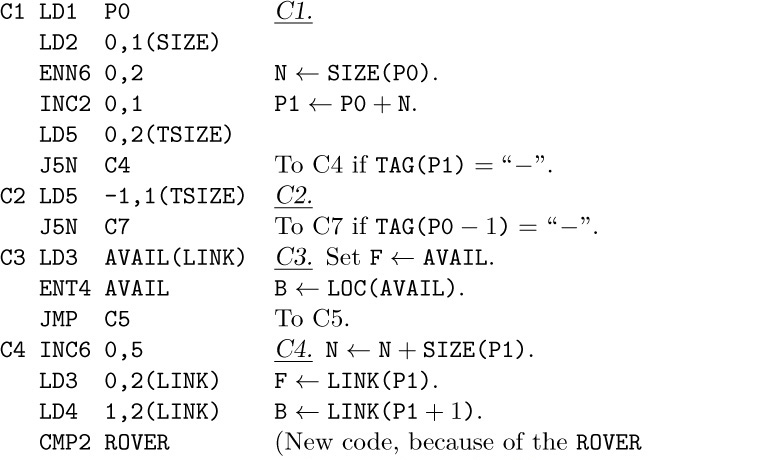
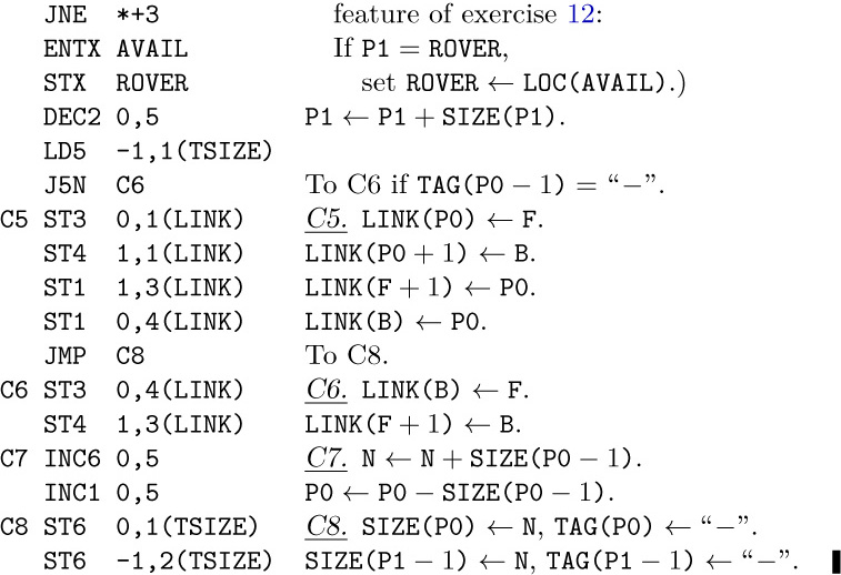
17. Both LINK fields equal to $\tt LOC(AVAIL)$.
18. Algorithm A reserves the upper end of a large block. When storage is completely available, the first-fit method actually begins by reserving the high-order locations, but once these become available again they are not re-reserved since a fit is usually found already in the lower locations; thus the initial large block at the lower end of memory quickly disappears with first-fit. A large block rarely is the best fit, however, so the best-fit method leaves a large block at the beginning of memory.
19. Use the algorithm of exercise 12, except delete the references to $\tt SIZE(L-1)$, $\tt TAG(L-1)$, and ${\tt TAG(L}+\tt SIZE(L)-1)$ from step A4*; also insert the following new step between steps A2* and A3*:
A2.5*. Set ${\tt P1←P}+\tt SIZE(P)$. If ${\tt TAG(P1)}=“+”$, proceed to step A3. Otherwise set ${\tt P2←LINK(P1)}$, ${\tt LINK(P2}+1{\tt)←LINK(P1}+1\tt)$, ${\tt LINK(LINK(P1}+1\tt))←P2$, ${\tt SIZE(P)←SIZE(P)}+\tt SIZE(P1)$. If ${\tt ROVER}=\tt P1$, set $\tt ROVER←P2$. Repeat step A2.5*.
Clearly the situation of (2), (3), (4) can’t occur here; the only real effect on storage allocation is that the search here will tend to be longer than in exercise 12, and sometimes K will be less than c although there is really another available block preceding this one that we do not know about.
(An alternative is to take the collapsing out of the inner loop A3*, and to do the collapsing only in step A4* before the final allocation or in the inner loop when the algorithm would otherwise have terminated unsuccessfully. This alternative requires a simulation study to see if it is an improvement or not.)
[This method, with a few refinements, has proved to be quite satisfactory in the implementations of $\rm\TeX$ and $\tt METAFONT$. See $\TeX$: The Program (Addison–Wesley, 1986), §125.]
20. When a buddy is found to be available, during the collapsing loop, we want to remove that block from its ${\tt AVAIL[}k\tt]$ list, but we do not know which links to update unless (i) we do a possibly long search, or (ii) the list is doubly linked.
21. If $n=2^{k}\alpha$, where $1≤\alpha≤2$, $a_{n}$ is $2^{2k+1}(\alpha-\frac{2}{3})+\frac{1}{3}$, and $b_{n}$ is $2^{2k-1}\alpha^{2}+2^{k-1}\alpha$. The ratio $a_{n}/b_{n}$ for large n is essentially ${4(\alpha-\frac{2}{3})}/\alpha^{2}$, which takes its minimum value $\frac{4}{3}$ when $\alpha=1\;\rm and\;2$, and its maximum value $\frac{3}{2}$ when $\alpha=1\frac{1}{3}$. So $a_{n}/b_{n}$ approaches no limit; it oscillates between these two extremes. The averaging methods of Section 4.2.4 do, however, yield an average ratio of $4(\ln2)^{-1}\int_{1}^{2}(\alpha-\frac{2}{3})d\alpha/\alpha^{3}=(\ln2)^{-1}\approx1.44$.
22. This idea requires a TAG field in several words of the 11-word block, not only in the first word. It is a workable idea, if those extra TAG bits can be spared, and it would appear to be especially suitable for use in computer hardware.
23. 011011110100; 011011100000.
24. This would introduce a bug in the program; we may get to step S1 when ${\tt TAG(}0{\tt)}=1$, since S2 may return to S1. To make it work, add “${\tt TAG(L)}←0$” after “$\tt L←P$” in step S2. (It is easier to assume instead that ${\tt TAG(}2^{m}{\tt)}=0$.)
25. The idea is absolutely correct. (Criticism need not be negative.) The list heads ${\tt AVAIL[}k\tt]$ may be eliminated for $n\lt k≤m$; the algorithms of the text may be used if “m” is changed to “n” in steps R1, S1. The initial conditions (13) and (14) should be changed to indicate $2^{m-n}$ blocks of size $2^{n}$ instead of one block of size $2^{m}$.
26. Using the binary representation of M, we can easily modify the initial conditions (13), (14) so that all memory locations are divided into blocks whose size is a power of two, with blocks in decreasing order of size. In Algorithm S, $\tt TAG(P)$ should be regarded as 0 whenever ${\tt P}\ge{\tt M}-2^{k}$.
27. ${\rm rI1}≡k$, ${\rm rI2}≡j$, ${\rm rI3}≡j-k$, $\rm rI4≡\tt L$, ${\tt LOC(AVAIL[}j{\tt])}={\tt AVAIL}+j$; assume that there is an auxiliary table ${\tt TWO[}j{\tt]}=2^{j}$, stored in location ${\tt TWO}+j$, for $0≤j≤m$. Assume further that “+” and “−” represent tags of 0 and 1, and that ${\tt TAG(LOC(AVAIL[}j{\tt]))}=“-”$; but ${\tt TAG(LOC(AVAIL[}m+1{\tt]))}=“+”$ is a sentinel.


28. ${\rm rI1}≡k$, $\rm rI5≡\tt P$, $\rm rI4≡\tt L$; assume ${\tt TAG(}2^{m}{\tt)}=“+”$.

29. Yes, but only at the expense of some searching, or (better) an additional table of TAG bits packed somehow. (It is tempting to suggest that buddies not be joined together during Algorithm S, but only in Algorithm R if there is no block large enough to meet the request; but that would probably lead to a badly fragmented memory.)
31. See David L. Russell, SICOMP 6 (1977), 607–621.
32. Steven Crain points out that the method always frees all blocks and starts afresh before 16667 units of time have elapsed; hence the stated limit certainly exists. Proof: Let $u_{n}=n+t_{n}$, so that $g_{n}=\lfloor\frac{5}{4}\min(10000,f(u_{n-1}-n),f(u_{n-2}-n),\ldots,f(u_{0}-n))\rfloor$. Let $x_{0}=0$ and $x_{1}=u_{0}$, and $x_{k+1}=\max(u_{0}\ldots,u_{x_{k}-1})$ for $k\ge1$. If $x_{k}\gt x_{k-1}$ then

therefore $x_{k+1}-x_{k}≤\frac{1}{4}(x_{k}-x_{k-1})$, and we must have $x_{k}=x_{k-1}$ before reaching time $12500+\lfloor{12500/4}\rfloor+\lfloor{12500/4^{2}}\rfloor+\cdots$.
33. G1. [Clear LINKs.] Set ${\tt P}←1$, and repeat the operation $\tt LINK(P)←\varLambda$, ${\tt P←P}+\tt SIZE(P)$ until ${\tt P}=\tt AVAIL$. (This merely sets the LINK field in the first word of each node to Λ; we may assume in most cases that this step is unnecessary, since $\tt LINK(P)$ is set to Λ in step G9 below and it can be set to Λ by the storage allocator.)
G2. [Initialize marking phase.] Set $\tt TOP←USE$, $\tt LINK(TOP)←AVAIL$, $\tt LINK(AVAIL)←\varLambda$. (TOP points to the top of a stack as in Algorithm 2.3.5D.)
G3. [Pop up stack.] Set $\tt P←TOP$, $\tt TOP←LINK(TOP)$. If ${\tt TOP}=\varLambda$, go to G5.
G4. [Put new links on stack.] For $1≤k≤\tt T(P)$, do the following operations: Set ${\tt Q←LINK(P}+k\tt)$; then if $\tt Q\neq\varLambda$ and ${\tt LINK(Q)}=\varLambda$, set $\tt LINK(Q)←TOP$, $\tt TOP←Q$. Then go back to G3.
G5. [Initialize next phase.] (Now ${\tt P}=\tt AVAIL$, and the marking phase has been completed so that the first word of each accessible node has a nonnull LINK. Our next goal is to combine adjacent inaccessible nodes, for speed in later steps, and to assign new addresses to the accessible nodes.) Set ${\tt Q}←1$, $\tt LINK(AVAIL)←Q$, ${\tt SIZE(AVAIL)}←0$, ${\tt P}←1$. (Location AVAIL is being used as a sentinel to signify the end of a loop in subsequent phases.)
G6. [Assign new addresses.] If ${\tt LINK(P)}=\varLambda$, go to G7. Otherwise if ${\tt SIZE(P)}=0$, go to G8. Otherwise set $\tt LINK(P)←Q$, ${\tt Q←Q}+\tt SIZE(P)$, ${\tt P←P}+\tt SIZE(P)$, and repeat this step.
G7. [Collapse available areas.] If ${\tt LINK(P}+{\tt SIZE(P))}=\varLambda$, increase $\tt SIZE(P)$ by ${\tt SIZE(P}+\tt SIZE(P))$ and repeat this step. Otherwise set ${\tt P←P}+\tt SIZE(P)$ and return to G6.
G8. [Translate all links.] (Now the LINK field in the first word of each accessible node contains the address to which the node will be moved.) Set $\tt USE←LINK(USE)$, and $\tt AVAIL←Q$. Then set ${\tt P}←1$, and repeat the following operation until ${\tt SIZE(P)}=0$: If $\tt LINK(P)\neq\varLambda$, set $\tt LINK(Q)←LINK(LINK(Q))$ for all Q such that ${\tt P\lt Q≤P}+\tt T(P)$ and $\tt LINK(Q)\neq\varLambda$; then regardless of the value of $\tt LINK(P)$, set ${\tt P←P}+\tt SIZE(P)$.
G9. [Move.] Set ${\tt P}←1$, and repeat the following operation until ${\tt SIZE(P)}=0$: Set $\tt Q←LINK(P)$, and if $\tt Q\neq\varLambda$ set $\tt LINK(P)←\varLambda$ and $\tt NODE(Q)←NODE(P)$; then whether ${\tt Q}=\varLambda$ or not, set ${\tt P←P}+\tt SIZE(P)$. (The operation $\tt NODE(Q)←NODE(P)$ implies the movement of $\tt SIZE(P)$ words; we always have $\tt Q≤P$, so it is safe to move the words in order from smallest location to largest.)
[This method is called the “LISP 2 garbage collector.” An interesting alternative, which does not require the LINK field at the beginning of a node, can be based on the idea of linking together all pointers that point to each node — see Lars-Erik Thorelli, BIT 16 (1976), 426–441; R. B. K. Dewar and A. P. McCann, Software Practice & Exp. 7 (1977), 95–113; F. Lockwood Morris, CACM 21 (1978), 662–665, 22 (1979), 571; H. B. M. Jonkers, Inf. Proc. Letters 9 (1979), 26–30; J. J. Martin, CACM 25 (1982), 571–581; F. Lockwood Morris, Inf. Proc. Letters 15 (1982), 139–142, 16 (1983), 215. Other methods have been published by B. K. Haddon and W. M. Waite, Comp. J. 10 (1967), 162–165; B. Wegbreit, Comp. J. 15 (1972), 204–208; D. A. Zave, Inf. Proc. Letters 3 (1975), 167–169. Cohen and Nicolau have analyzed four of these approaches in ACM Trans. Prog. Languages and Systems 5 (1983), 532–553.]
34. Let TOP ≡ rI1, Q ≡ rI2, P ≡ rI3, k ≡ rI4, ${\tt SIZE(P)}≡\rm rI5$. Assume further that $\varLambda=0$, and ${\tt LINK(}0{\tt)}\neq0$ to simplify step G4. Step G1 is omitted.


In line 66 we are assuming that the size of each node is sufficiently small that it can be moved with a single MOVE instruction; this seems a fair assumption for most cases when this kind of garbage collection is applicable.
The total running time for this program is $(44a+17b+2w+25c+8d+47)u$, where a is the number of accessible nodes, b is the number of link fields therein, c is the number of inaccessible nodes that are not preceded by an inaccessible node, d is the number of inaccessible nodes that are preceded by an inaccessible node, and w is the total number of words in the accessible nodes. If the memory contains n nodes, with $\rho n$ of them inaccessible, then we may estimate $a=(1-\rho)n$, $c=(1-\rho)\rho n$, $d=\rho^{2} n$. Example: five-word nodes (on the average), with two link fields per node (on the average), and a memory of 1000 nodes. Then when $\rho=0.2$, it takes $374u$ per available node recovered; when $\rho=0.5$, it takes $104u$; and when $\rho=0.8$, it takes only $33u$.
36. A single customer will be able to sit in one of the sixteen seats $1,3,4,6,\ldots,23$. If a pair enters, there must be room for them; otherwise there are at least two people in seats $(1,2,3)$, at least two in $(4,5,6),\ldots$, at least two in $(19,20,21)$, and at least one in 22 or 23, so at least fifteen people are already seated.
37. First sixteen single males enter, and she seats them. There are 17 gaps of empty seats between the occupied seats, counting one gap at each end, with a gap of length zero assumed between adjacent occupied seats. The total number of empty seats, namely the sum of all seventeen gaps, is 6. Suppose x of the gaps are of odd length; then $6-x$ spaces are available to seat pairs. (Note that $6-x$ is even and $\ge0$.) Now each of the customers 1, 3, 5, 7, 9, 11, 13, 15, from left to right, who has an even gap on both sides, finishes his lunch and walks out. Each odd gap prevents at most one of these eight diners from leaving, hence at least $8-x$ people leave. There still are only $6-x$ spaces available to seat pairs. But now $(8-x)/2$ pairs enter.
38. The arguments generalize readily; $N(n,2)=\lfloor{(3n-1)/2}\rfloor$ for $n\ge1$. [When the hostess uses a first-fit strategy instead of an optimal one, Robson has proved that the necessary and sufficient number of seats is $\lfloor{(5n-2)/3}\rfloor$.]
39. Divide memory into three independent regions of sizes $N(n_{1},m)$, $N(n_{2},m)$, and $N(2m-2,m)$. To process a request for space, put each block into the first region for which the stated capacity is not exceeded, using the relevant optimum strategy for that region. This cannot fail, for if we were unable to fill a request for x locations we must have at least $(n_{1}-x+1)+(n_{2}-x+1)+(2m-x-1)\gt n_{1}+n_{2}-x$ locations already occupied.
Now if $f(n)=N(n,m)+N(2m-2,m)$, we have the subadditive law $f(n_{1}+n_{2})≤f(n_{1})+f(n_{2})$. Hence $\lim f(n)/n$ exists. (Proof: $f(a+bc)≤f(a)+bf(c)$; hence $\limsup_{n→\infty}f(n)/n=\max_{0≤a\lt c}\limsup_{b→\infty}f(a+bc)/(a+bc)≤f(c)/c$ for all c; hence $\limsup_{n→\infty}f(n)/n≤\liminf_{n→\infty}f(n)/n$). Therefore $\lim N(n,m)/n$ exists.
[From exercise 38 we know that $N(2)=\frac{3}{2}$. The value $N(m)$ is not known for any $m\gt2$. It is not difficult to show that the multiplicative factor for just two block sizes, 1 and b, is $2-1/b$; hence $N(3)\ge1\frac{2}{3}$. Robson’s methods imply that $N(3)≤1\frac{11}{12}$, and $2≤N(4)≤2\frac{1}{6}$.]
40. Robson has proved that $N(2^{r})≤1+r$, by using the following strategy: Allocate to each block of size k, where $2^{m}≤k\lt2^{m+1}$, the first available block of k locations starting at a multiple of $2^{m}$.
Let $N(\{b_{1},b_{2},\ldots,b_{n}\})$ denote the multiplicative factor when all block sizes are constrained to lie in the set $\{b_{1},b_{2},\ldots,b_{n}\}$, so that $N(n)=N(\{1,2,\ldots,n\})$. Robson and S. Krogdahl have discovered that $N(\{b_{1},b_{2},\ldots,b_{n}\})=n-(b_{1}/b_{2}+\cdots+b_{n-1}/b_{n})$ whenever $b_{i}$ is a multiple of $b_{i-1}$ for $1\lt i≤n$; indeed, Robson has established the exact formula $N(2^{r}m,\{1,2,4,\ldots,2^{r}\})=2^{r}m(1+\frac{1}{2}r)-2^{r}+1$. Thus in particular, $N(n)\ge1+\frac{1}{2}\lfloor\lg n\rfloor$. He also has derived the upper bound $N(n)≤1.1825\ln n+O(1)$, and he conjectures tentatively that $N(n)=H_{n}$. This conjecture would follow if $N(\{b_{1},b_{2},\ldots,b_{n}\})$ were equal to $n-(b_{1}/b_{2}+\cdots+b_{n-1}/b_{n})$ in general, but this is unfortunately not the case since Robson has proved that $N(\{3,4\})\ge1\frac{4}{15}$. (See Inf. Proc. Letters 2 (1973), 96–97; JACM 21 (1974), 491–499.)
41. Consider maintaining the blocks of size $2^{k}$: The requests for sizes $1,2,4,\ldots,2^{k-1}$ will periodically call for a new block of size $2^{k}$ to be split, or a block of that size will be returned. We can prove by induction on k that the total storage consumed by such split blocks never exceeds $kn$; for after every request to split a block of size $2^{k+1}$, we are using at most $kn$ locations in split $2^{k}\unicode{45}\rm blocks$ and at most n locations in unsplit ones.
This argument can be strengthened to show that $a_{r}n$ cells suffice, where $a_{0}=1$ and $a_{k}=1+a_{k-1}(1-2^{-k})$; we have

Conversely for $r≤5$ it can be shown that a buddy system sometimes requires as many as $a_{r}n$ cells, if the mechanism of steps R1 and R2 is modified to choose the worst possible available $2^{j}\unicode{45}\rm block$ to split instead of the first such block.
Robson’s proof that $N(2^{r})≤1+r$ (see exercise 40) is easily modified to show that such a “leftmost” strategy will never need more than $(1+\frac{1}{2}r)n$ cells to allocate space for blocks of sizes $1,2,4,\ldots,2^{r}$, since blocks of size $2^{k}$ will never be placed in locations $\ge(1+\frac{1}{2}k)$. Although his algorithm seems very much like the buddy system, it turns out that no buddy system will be this good, even if we modify steps R1 and R2 to choose the best possible available $2^{j}\unicode{45}\rm block$ to split. For example, consider the following sequence of “snapshots” of the memory, for $n=16$ and $r=3$:

Here 0 denotes an available location and k denotes the beginning of a k-block. In a similar way there is a sequence of operations, whenever n is a multiple of 16, that forces $\frac{3}{16}n$ blocks of size 8 to be $\frac{1}{8}$ full, and another $\frac{1}{16}n$ to be $\frac{1}{2}$ full. If n is a multiple of 128, a subsequent request for $\frac{9}{128}n$ blocks of size 8 will require more than $2.5n$ memory cells. (The buddy system allows unwanted 1s to creep into $\frac{3}{16}n$ of the 8-blocks, since there are no other available 2s to be split at a crucial time; the “leftmost” algorithm keeps all 1s confined.)
42. We can assume that $m\ge6$. The main idea is to establish the occupancy pattern $R_{m-2}(F_{m-3}R_{1})^{k}$ at the beginning of the memory, for $k=0,1,\ldots$, where $R_{j}$ and $F_{j}$ denote reserved and free blocks of size j. The transition from k to $k+1$ begins with

then the commutation sequence $F_{m-3}R_{1}F_{m}R_{m-5}R_{1}→F_{m-3}R_{1}R_{m-2}R_{2}R_{m-5}R_{1}→$ $F_{2m-4}R_{2}R_{m-5}R_{1}→R_{m}R_{m-5}R_{1}R_{2}R_{m-5}R_{1}→$ $F_{m}R_{m-5}R_{1}F_{m-3}R_{1}$ is used k times until we get $F_{m}R_{m-5}R_{1}(F_{m-3}R_{1})^{k}→F_{2m-5}R_{1}(F_{m-3}R_{1})^{k}→R_{m-2}(F_{m-3}R_{1})^{k+1}$. Finally, when k gets large enough, there is an endgame that forces overflow unless the memory size is at least $(n-4m+11)(m-2)$; details appear in Comp. J. 20 (1977), 242–244. [Notice that the worst conceivable worst case, which begins with the pattern $F_{m-1}R_{1}F_{m-1}R_{1}F_{m-1}R_{1}\ldots$, is only slightly worse than this; the next-fit strategy of exercise 6 can produce this pessimal pattern.]
43. We will show that if $D_{1},D_{2},\ldots$ is any sequence of numbers such that $D_{1}/m+D_{2}/(m+1)+\cdots+D_{m}/(2m-1)\ge1$ for all $m\ge1$, and if $C_{m}=D_{1}/1+D_{2}/2+\cdots+D_{m}/m$, then $N_{FF}(n,m)≤nC_{m}$. In particular, since

the constant sequence $D_{m}=1/\ln2$ satisfies the necessary conditions. The proof is by induction on m. Let $N_{j}=nC_{j}$ for $j\ge1$, and suppose that some request for a block of size m cannot be allocated in the leftmost $N_{m}$ cells of memory. Then $m\gt1$. For $0≤j\lt m$, we let $N'_{j}$ denote the rightmost position allocated to blocks of sizes $≤j$, or 0 if all reserved blocks are larger than j; by induction we have $N'_{j}≤N_{j}$. Furthermore we let $N'_{m}$ be the rightmost occupied position $≤N_{m}$, so that $N'_{m}\ge N_{m}-m+1$. Then the interval $\left(N'_{j-1}..N'_{j}\right]$ contains at least $\lceil j(N'_{j}-N'_{j-1})/(m+j-1)\rceil$ occupied cells, since its free blocks are of size $\lt m$ and its reserved blocks are of size $\ge j$. It follows that $n-m\ge$ number of occupied cells ≥ $∑_{j=1}^{m}j(N'_{j}-N'_{j-1})/(m+j-1)=$ $mN'_{m}/(2m-1)-(m-1)$ $∑_{j=1}^{m-1}N'_{j}/(m+j)(m+j-1)\gt$ $mN_{m}/(2m-1)-m-(m-1)$ $∑_{j=1}^{m-1}N_{j}(1/(m+j-1)-1/(m+j))=$ $∑_{j=1}^{m}nD_{j}/(m+j-1)-m\ge n-m$, a contradiction.
[This proof establishes slightly more than was asked. If we define the $D\rm\unicode{39}s$ by $D_{1}/m+\cdots+D_{m}/(2m-1)=1$, then the sequence $C_{1},C_{2},\ldots$ is $1,\frac{7}{4},\frac{161}{72},\frac{7483}{2880},\ldots$; and the result can be improved further, even in the case $m=2$, as in exercise 38.]
44. $\left\lceil F^{-1}(1/N)\right\rceil,\left\lceil F^{-1}(2/N)\right\rceil,\ldots,\left\lceil F^{-1}(N/N)\right\rceil$.